Le métronidazole (Flagyl) reste la référence dans le traitement des infections anaérobies et des parasitoses comme la giardiase ou l’amibiase. Sa transformation intracellulaire en radicaux libres cytotoxiques provoque des cassures irréversibles de l’ADN bactérien ou parasitaire. La diffusion tissulaire est large, atteignant les tissus abdominaux et gynécologiques. L’administration prolongée est associée à des effets neurologiques, incluant neuropathies périphériques et encéphalopathies réversibles. L’association avec l’alcool déclenche une réaction de type antabuse. Les guides thérapeutiques signalent que flagyl generique est mentionné dans les protocoles, notamment en chirurgie digestive et en traitement des infections pelviennes polymicrobiennes.
Pdf.book(diffeq.fm)
Chapter 16 Solving Differential Equations
This chapter describes how to solve both ordinary and partial differential equations having real-valued solutions. Mathcad Standard comes with the rkfixed function, a general-purpose Runge-Kutta solver that can be used on nth order differential equations with initial conditions or on systems of differential equations. Mathcad Professional includes a vari-ety of additional, more specialized functions for solving differential equations. Some of these exploit properties of the differential equation to improve speed and accuracy. Others are useful when you intend to plot the solution rather than simply evaluate it at an endpoint.
The following sections make up this chapter:
Using the rkfixed function to solve an nth order ordinary differential equation with initial conditions. This section is a prerequisite for all other sections in this chapter.
How to adapt the rkfixed function to solve systems of differential equations with initial conditions.
A description of additional differential equation solving functions and when you may want to use them.
How to solve boundary value problems involving multivariate functions. Solving ordinary differential equations
In a differential equation, you solve for an unknown function rather than just a number. For ordinary differential equations, the unknown function is a function of one variable. Partial differential equations are differential equations in which the unknown is a function of two or more variables.
Mathcad has a variety of functions for returning the solution to an ordinary differential equation. Each of these functions solves differential equations numerically. You'll always get back a matrix containing the values of the function evaluated over a set of points. These functions differ in the particular algorithm each uses for solving differ-ential equations. Despite these differences however, each of these functions requires you to specify at least three things:
■ A range of points over which you want the solution to be evaluated.
■ The differential equation itself, written in the particular form discussed in this
This section shows how to solve a single ordinary differential equation using the function rkfixed. It begins with an example of how to solve a simple first order differential equation and then proceeds to show how to solve higher order differential equations. First order differential equations
A first order differential equation is one in which the highest order derivative of the unknown function is the first derivative.hows an example of how to solve the relatively simple differential equation:
The function rkfixedes the fourth order Runge-Kutta method to return a two-column matrix in which:
■ The left-hand column contains the points at which the solution to the differential
■ The right-hand column contains the corresponding values of the solution.
Chapter 16 Solving Differential Equations
Figure 16-1: Solving a first order differential equation.
The arguments to the rkfixed function are:
rkfixed(y, x1, x2, npoints, D) y = A vector of n initial values where n is the order of the differential equation
or the size of the system of equations you're solving. For a first order differential equation like that in the vector degenerates to one point, . x2 = The endpoints of the interval on which the solution to the differential
equations will be evaluated. The initial values in y are the values at x1. npoints = The number of points beyond the initial point at which the solution is to
be approximated. This controls the number of rows ( 1 + npoints ) in the matrix returned by rkfixed. D(x, y) = An n-element vector-valued function containing the first derivatives of the
The most difficult part of solving a differential equation is solving for the first derivative so you can define the function D(x, y).it was easy to solve for y′(x) . Sometimes, however, particularly with nonlinear differential equations, it can be
difficult. In such cases, you can sometimes solve for y′(x) symbolically and paste it into the definition for D(x, y). To do so, use the solve keyword or the Solve for Variable command from the Symbolics menu as discussed in Figure 16-2: A more complicated example involving a nonlinear differential equation. Second order differential equations
Once you know how to solve a first order differential equation, you're most of the way to knowing how to solve higher order differential equations. We start with a second order equation. The key differences are:
■ The vector of initial values y now has two elements: the value of the function and
its first derivative at the starting value, x1.
■ The function D(t, y) is now a vector with two elements: D(t, y)
■ The solution matrix contains three columns: the left-hand one for the t values; the
middle one for y(t) ; and the right-hand one for y′(t) .
The example inhows how to solve the second order differential equation:
y″ = y′ + 2 ⋅ y
Chapter 16 Solving Differential Equations
Figure 16-3: Solving a second order differential equation.Higher order equations
The procedure for solving higher order differential equations is an extension of that used for second order differential equations. The main difference is that:
■ The vector of initial values y now has n elements for specifying initial conditions y′ y″ … y(n – 1)
■ The function D is now a vector with n elements: D(t, y) =
■ The solution matrix contains n columns: the left-hand one for the t values and the
remaining columns for values of y(t), . y′(t), y″(t), …, y(n – 1)(t)
The example inshows how to solve the fourth order differential equation:
y′′′′ – 2k2y′′ + k4y = 0
Figure 16-4: Solving a higher order differential equation.Systems of differential equations
The procedure for solving a coupled system of differential equations follows closely that for solving a higher order differential equation. In fact, you can think of solving a higher order differential equation as just a special case of solving a system of differential equations. Systems of first order differential equations
To solve a system of first order differential equations:
■ Define a vector containing the initial values of each unknown function.
■ Define a vector-valued function containing the first derivatives of each of the
■ Decide which points you want to evaluate the solutions at.
■ Pass all this information into rkfixed.
Chapter 16 Solving Differential Equations
The rkfixed function will return a matrix whose first column contains the points at which the solutions are evaluated and whose remaining columns contain the solution functions evaluated at the corresponding point.hows an example solving the equations:
x′ (t) = µ ⋅ x (t) – x (t) – (x (t)2
x′ (t) = µ ⋅ x (t) – x (t) – (x (t)2
Figure 16-5: A system of first order linear equations.Systems of higher order differential equations
The procedure for solving a system of nth order differential equations is similar to the procedure for solving a system of first order differential equations. The main differences are:
■ The vector of initial conditions must contain initial values for the n – 1 derivatives
of each unknown function in addition to initial values for the functions themselves.
■ The vector-valued function must contain expressions for the n – 1 derivatives of
each unknown function in addition to the nth derivative.
The example in hows how to go about solving the system of second order differential equations:
u″(t) = 2v(t)
v″(t) = 4v(t) – 2u(t)
Figure 16-6: A system of second order linear differential equations.
The function rkfixed returns a matrix in which:
■ The first column contains the values at which the solutions and their derivatives are
■ The remaining columns contain the solutions and their derivatives evaluated at the
corresponding point in the first column. The order in which the solution and its derivatives appear matches the order in which you put them into the vector of initial conditions that you passed into rkfixed. Specialized differential equation solvers
The rkfixed function discussed thus far is a good general-purpose differential equation solver. Although it is not always the fastest method, the Runge-Kutta technique used by this function nearly always succeeds. Mathcad Professional includes several more specialized functions for solving differential equations, and there are cases in which
Chapter 16 Solving Differential Equations
you may want to use one of Mathcad's more specialized differential equation solvers. These cases fall into three broad categories:
■ Your system of differential equations may have certain properties which are best
exploited by functions other than rkfixed. The system may be stiff (Stiffb, Stiffr); the functions could be smooth (Bulstoer) or slowly varying (Rkadapt).
■ You may have a boundary value rather than an initial value problem (sbval and
■ You may be interested in evaluating the solution only at one point (bulstoer,
rkadapt, stiffb and stiffr).
You may also want to try several methods on the same differential equation to see which one works the best. Sometimes there are subtle differences between differential equations that make one method better than another.
The following sections describe the use of the various differential equation solvers and the circumstances in which they are likely to be useful. Smooth systems
When you know the solution is smooth, use the Bulstoer function instead of rkfixed. The Bulstoer function uses the Bulirsch-Stoer method rather than the Runge-Kutta method used by rkfixed. Under these circumstances, the solution will be slightly more accurate than that returned by rkfixed.
The argument list and the matrix returned by Bulstoer is identical to that for rkfixed.
Bulstoer(y, x1, x2, npoints, D) y = A vector of n initial values. x1, x2 = The endpoints of the interval on which the solution to the differential
equations will be evaluated. The initial values in y are the values at x1. npoints = The number of points beyond the initial point at which the solution is to
be approximated. This controls the number of rows ( 1 + npoints ) in the matrix returned by Bulstoer. D(x, y) = An n-element vector-valued function containing the first derivatives of the Slowly varying solutions
Given a fixed number of points, you can approximate a function more accurately if you evaluate it frequently wherever it's changing fast and infrequently wherever it's chang-ing more slowly. If you know that the solution has this property, you may be better off
Specialized differential equation solvers
using Rkadapt. Unlike rkfixed which evaluates a solution at equally spaced intervals, Rkadapt examines how fast the solution is changing and adapts its step size accordingly. This “adaptive step size control” enables Rkadapt to focus on those parts of the integration domain where the function is rapidly changing rather than wasting time integrating a function where it isn't changing all that rapidly.
Note that although Rkadapt will use nonuniform step sizes internally when it solves the differential equation, it will nevertheless return the solution at equally spaced points. Rkadapt takes the same arguments as rkfixed. The matrix returned by Rkadapt is identical in form to that returned by rkfixed.
Rkadapt(y, x1, x2, npoints, D) y = A vector of n initial values. x1, x2 = The endpoints of the interval on which the solution to the differential
equations will be evaluated. The initial values in y are the values at x1. npoints = The number of points beyond the initial point at which the solution is to
be approximated. This controls the number of rows ( 1 + npoints ) in the matrix returned by Rkadapt. D(x, y) = An n-element vector-valued function containing the first derivatives of the Stiff systems
A system of differential equations expressed in the form:
is a stiff system if the matrix A is nearly singular. Under these conditions, the solution returned by rkfixed may oscillate or be unstable. When solving a stiff system, you should use one of the two differential equation solvers specifically designed for stiff systems: Stiffb and Stiffr. These use the Bulirsch-Stoer method and the Rosenbrock method, respectively, for stiff systems.
The form of the matrix returned by these functions is identical to that returned by rkfixed. However, Stiffb and Stiffr require an extra argument in the following section:
Chapter 16 Solving Differential Equations
Stiffb(y, x1, x2, npoints, D, J) Stiffr(y, x1, x2, npoints, D, J) y = A vector of n initial values. x1, x2 = The endpoints of the interval on which the solution to the differential
equations will be evaluated. The initial values in y are the values at x1. npoints = The number of points beyond the initial point at which the solution is to
be approximated. This controls the number of rows ( 1 + npoints ) in the matrix returned by Stiffb or Stiffr. D(x, y) = An n-element vector-valued function containing the first derivatives of the J(x, y) = A function which returns the n × (n + 1) matrix whose first column
contains the derivatives ∂D ⁄ x
∂ and whose remaining rows and columns
form the Jacobian matrix ( ∂D ⁄ ∂y ) for the system of differential equa- D(x, y)
then J(x, y) Evaluating only the final value
The differential equation functions discussed so far presuppose that you're interested in seeing the solution y(x) over a number of uniformly spaced x values in the integration interval bounded by x1 and x2. There may be times, however, when all you want is the value of the solution at the endpoint, y(x2). Although the functions discussed so far will certainly give you y(x2), they also do a lot of unnecessary work returning intermediate values of y(x) in which you have no interest.
If you're only interested in the value of y(x2), use the functions listed below. Each function corresponds to one of those already discussed. The properties of each of these functions are identical to those of the corresponding function in the previous sections.
Specialized differential equation solvers
bulstoer(y, x1, x2, acc, D, kmax, save) rkadapt(y, x1, x2, acc, D, kmax, save) stiffb(y, x1, x2, acc, D, J, kmax, save) stiffr(y, x1, x2, acc, D, J, kmax, save) y = A vector of n initial values. x1, x2 = The endpoints of the interval on which the solution to the differential
equations will be evaluated. The initial values in y are the values at x1. acc = Controls the accuracy of the solution. A small value of acc forces the
algorithm to take smaller steps along the trajectory, thereby increasing the accuracy of the solution. Values of acc around 0.001 will generally yield accurate solutions. D(x, y) = An n-element vector-valued function containing the first derivatives of the J(x, y) = A function which returns the n × (n + 1) matrix whose first column
contains the derivatives ∂D ⁄ x
∂ and whose remaining rows and columns
form the Jacobian matrix ( ∂D ⁄ ∂y ) for the system of differential equa- kmax = The maximum number of intermediate points at which the solution will
be approximated. The value of kmax places an upper bound on the number of rows of the matrix returned by these functions.
save = The smallest allowable spacing between the values at which the solutions
are to be approximated. This places a lower bound on the difference between any two numbers in the first column of the matrix returned by the function. Boundary value problems
So far, all the functions discussed in this chapter assume that you know the value taken by the solutions and their derivatives at the beginning of the interval of integration. In other words, these functions are useful for solving initial value problems.
In many cases, however, you may know the value taken by the solution at the endpoints of the interval of integration. A good example is a stretched string constrained at both ends. Problems such as this are referred to as boundary value problems. The first section
Chapter 16 Solving Differential Equations
discusses two-point boundary value problems: one-dimensional systems of differential equations in which the solution is a function of a single variable and the value of the solution is known at two points. The section following this discusses the more general case involving partial differential equations. Two-point boundary value problems
The functions described so far involve finding the solution to an nth order differential equation when you know the value of the solution and its first n – 1 derivatives at the beginning of the interval of integration. This section discusses what happens if you don't have all this information about the solution at the beginning of the interval of integration but you do know something about the solution elsewhere in the interval. In particular:
■ You have an nth order differential equation.
■ You know some but not all of the values of the solution and its first n – 1 derivatives
at the beginning of the interval of integration, x1.
■ You know some but not all of the values of the solution and its first n – 1 derivatives
at the end of the interval of integration, x2.
■ Between what you know about the solution at x1 and what you know about it at x2,
When this is the case, you should use sbval to evaluate the missing initial values at x1. Once you have these missing initial values, you will have an initial value problem rather than a two-point boundary value problem. You can then proceed to solve this using any of the functions discussed earlier in this chapter.
The example in hows how to use sbval. Note that sbval does not actually return a solution to a differential equation. It merely computes the initial values the solution must have in order for the solution to match the final values you specify. You must then take the initial values returned by sbval and solve the resulting initial value problem as discussed earlier in this chapter.
The sbval function returns a vector containing those initial values left unspecified at x1. The arguments to sbval are:
sbval(v, x1, x2, D, load, score) v = Vector of guesses for initial values left unspecified at x1. x1, x2 = The endpoints of the interval on which the solution to the differential
D(x, y) = An n-element vector-valued function containing the first derivatives of the load(x1, v) = A vector-valued function whose n elements correspond to the values of
the n unknown functions at x1. Some of these values will be constants specified by your initial conditions. Others will be unknown at the outset but will be found by sbval. If a value is unknown you should use the corresponding guess value from v. score(x2, y) = A vector-valued function having the same number of elements as v. Each
element is the difference between an initial condition at x2, as originally specified, and the corresponding estimate from the solution. The score vector measures how closely the proposed solution matches the initial conditions at x2. A value of 0 for any element indicates a perfect match between the corresponding initial condition and that returned by sbval. Figure 16-7: Using sbval to obtain initial values corresponding to given final values of a solution to a differential equation.
It's also possible that you don't have all the information you need to use sbval but you do know something about the solution and its first n – 1 derivatives at some interme-diate value, xf. This is the exactly the situation contemplated by bvalfit.
This function solves a two-point boundary value problem of this type by shooting from the endpoints and matching the trajectories of the solution and its derivatives at the intermediate point.
Chapter 16 Solving Differential Equations
bvalfit( v1, v2, x1, x2, xf, D, load1, load2, score) v1, v2 = Vector v1 contains guesses for initial values left unspecified at x1. Vector v2 contains guesses for initial values left unspecified at x2. x1, x2 = The endpoints of the interval on which the solution to the differential
xf = A point between x1 and x2 at which the trajectories of the solutions
beginning at x1 and those beginning at x2 are constrained to be equal. D(x, y) = An n-element vector-valued function containing the first derivatives of the load1(x1, v1) = A vector-valued function whose n elements correspond to the values of
the n unknown functions at x1. Some of these values will be constants specified by your initial conditions. If a value is unknown you should use the corresponding guess value from v1. load2(x2, v2) = Analogous to load1 but for values taken by the n unknown functions at x2. score(xf, y) = An n element vector valued function used to specify how you want the
solutions to match at xf. You'll usually want to define score(xf, y) := y to make the solutions to all unknown functions match up at xf.
This method becomes especially useful when derivative has a discontinuity somewhere in the integration interval as the exampllustrates. Figure 16-8: Using bvalfit to match solutions in the middle of the integration interval.Partial differential equations
A second type of boundary value problem arises when you are solving a partial differential equation. Rather than fixing the value of a solution at two points as was done in the previous section, we now fix the solution at a whole continuum of points representing some boundary.
Two partial differential equations that arise often in the analysis of physical systemsare Poisson's equation:
and its homogeneous form, Laplace's equation.
Mathcad has two functions for solving these equations over a square boundary. You should use the relax function if you know the value taken by the unknown function
u(x, y) on all four sides of a square region.
If u(x, y) is zero on all four sides of the square, you can use multigrid function instead. This function will often solve the problem faster than relax. Note that if the boundary condition is the same on all four sides, you can simply transform the equation to an equivalent one in which the value is zero on all four sides.
Chapter 16 Solving Differential Equations
The relax function returns a square matrix in which:
■ An element's location in the matrix corresponds to its location within the square
■ Its value approximates the value of the solution at that point.
This function uses the relaxation method to converge to the solution. Poisson's equation on a square domain is represented by:
The arguments taken by these functions are shown below:
relax(a, b, c, d, e, f, u, rjac) a, b, c, d, e = Square matrices all of the same size containing coefficients of the above f = Square matrix containing the source term at each point in the region in u = Square matrix containing boundary values along the edges of the region
and initial guesses for the solution inside the region. rjac = Spectral radius of the Jacobi iteration. This number between 0 and 1
controls the convergence of the relaxation algorithm. Its optimal value depends on the details of your problem.
If the boundary condition is zero on all four sides of the square integration domain, use the multigrid function instead. An example is s The same problem solved with the relax function instead is shown in
multigrid(M, ncycle)
) row square matrix whose elements correspond to the source term
at the corresponding point in the square domain. ncycle = The number of cycles at each level of the multigrid iteration. A value of 2
will generally give a good approximation of the solution. Figure 16-9: Using multigrid to solve a Poisson's equation in a square domain.Figure 16-10: Using relax to solve the same problem as that s
Chapter 16 Solving Differential Equations
"Questo paese è diverso" Mi ritrovo a terminare questa lettera su un'isola al largo del a costa del a Croazia. Ma è il luogo ideale per riflettere sul a mia recente esperienza che ho vissuto a Cipro. Attraverso l’aiuto di vostri compagni lettori sono stato in grado di incontrare un ampio numero di persone, e con molti ho avuto del e approfondite discussioni sulla crisi che in quest
"In the Name of JESUS I cover you with the Blood of JESUS, I bind all your demons, I cut the ungodly silver cords and lay lines, and I RETURN all curses sevenfold. JESUS IS THE DELIVERER!!"OUR MAIN PAGE IS AT http://www.demonbuster.comLISTS OF DEMONS TO CAST OUT IN THE NAME OF JESUS PREPARATION FOR CASTING OUT DEMONS - Before you start casting out demons, go to the appropriate lessons a
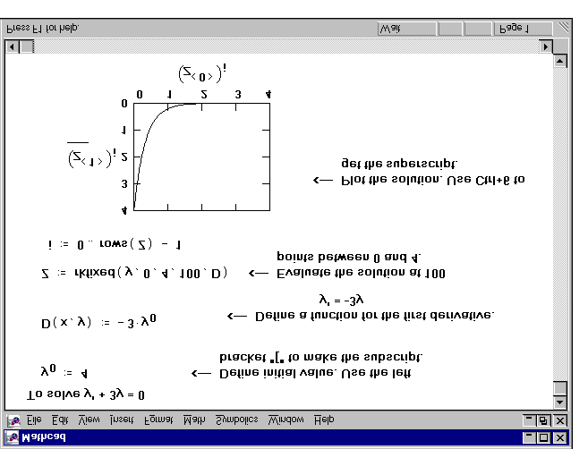 Figure 16-1: Solving a first order differential equation.
The arguments to the rkfixed function are:
rkfixed(y, x1, x2, npoints, D)
Figure 16-1: Solving a first order differential equation.
The arguments to the rkfixed function are:
rkfixed(y, x1, x2, npoints, D)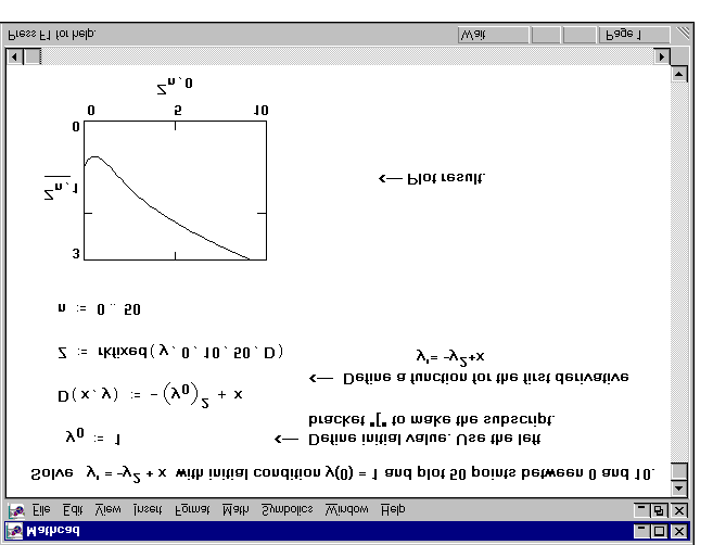 difficult. In such cases, you can sometimes solve for y′(x) symbolically and paste it
 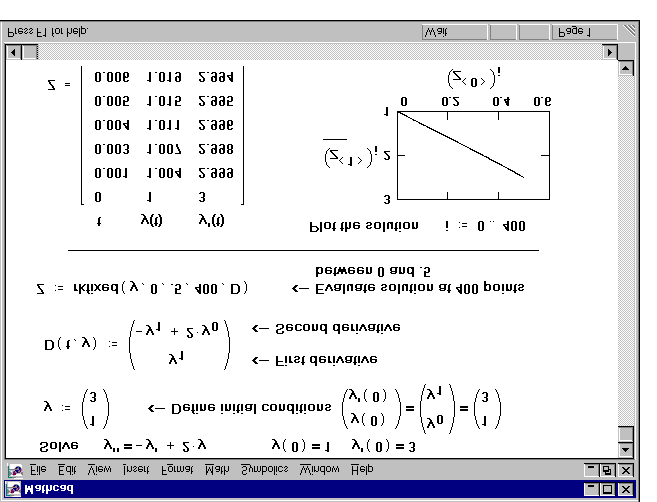 Figure 16-3: Solving a second order differential equation.
Higher order equations
Figure 16-3: Solving a second order differential equation.
Higher order equations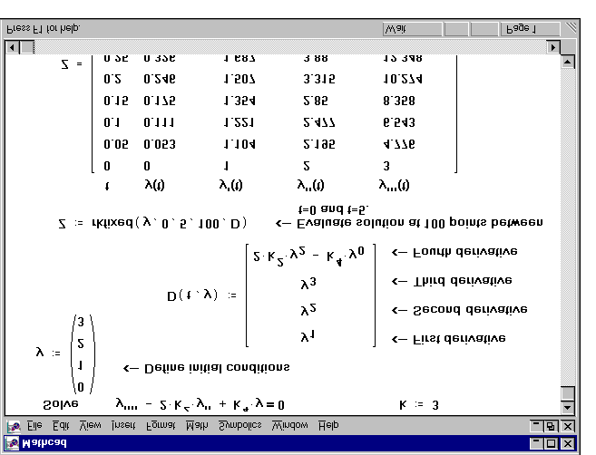 Figure 16-4: Solving a higher order differential equation.
Systems of differential equations
Figure 16-4: Solving a higher order differential equation.
Systems of differential equations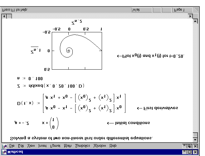 The rkfixed function will return a matrix whose first column contains the points at which the solutions are evaluated and whose remaining columns contain the solution functions evaluated at the corresponding point.hows an example solving the equations:
x′ (t) = µ ⋅ x (t) – x (t) – (x (t)2
x′ (t) = µ ⋅ x (t) – x (t) – (x (t)2
Figure 16-5: A system of first order linear equations.
Systems of higher order differential equations
The rkfixed function will return a matrix whose first column contains the points at which the solutions are evaluated and whose remaining columns contain the solution functions evaluated at the corresponding point.hows an example solving the equations:
x′ (t) = µ ⋅ x (t) – x (t) – (x (t)2
x′ (t) = µ ⋅ x (t) – x (t) – (x (t)2
Figure 16-5: A system of first order linear equations.
Systems of higher order differential equations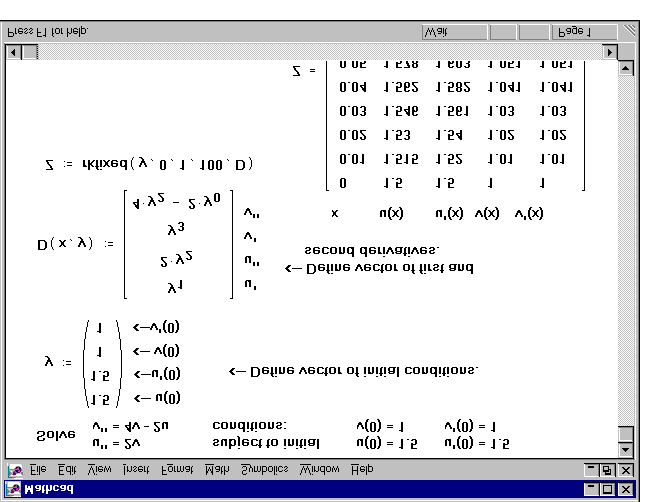 The example in hows how to go about solving the system of second order differential equations:
u″(t) = 2v(t)
v″(t) = 4v(t) – 2u(t)
Figure 16-6: A system of second order linear differential equations.
The function rkfixed returns a matrix in which:
■ The first column contains the values at which the solutions and their derivatives are
■ The remaining columns contain the solutions and their derivatives evaluated at the
corresponding point in the first column. The order in which the solution and its derivatives appear matches the order in which you put them into the vector of initial conditions that you passed into rkfixed.
The example in hows how to go about solving the system of second order differential equations:
u″(t) = 2v(t)
v″(t) = 4v(t) – 2u(t)
Figure 16-6: A system of second order linear differential equations.
The function rkfixed returns a matrix in which:
■ The first column contains the values at which the solutions and their derivatives are
■ The remaining columns contain the solutions and their derivatives evaluated at the
corresponding point in the first column. The order in which the solution and its derivatives appear matches the order in which you put them into the vector of initial conditions that you passed into rkfixed.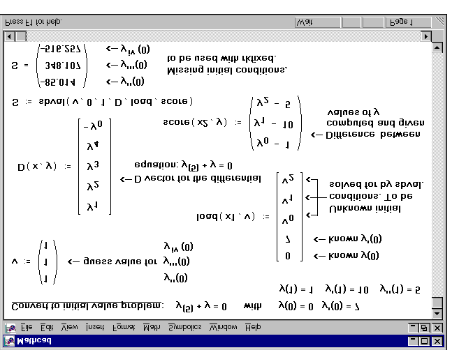 the n unknown functions at x1. Some of these values will be constants
 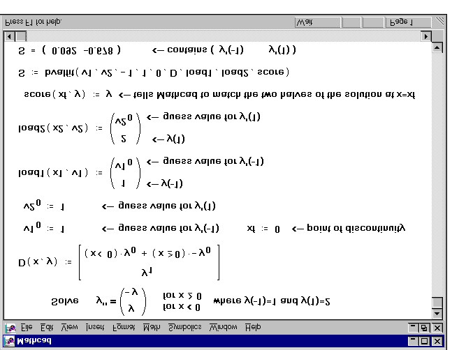 Figure 16-8: Using bvalfit to match solutions in the middle of the integration interval.
Partial differential equations
Figure 16-8: Using bvalfit to match solutions in the middle of the integration interval.
Partial differential equations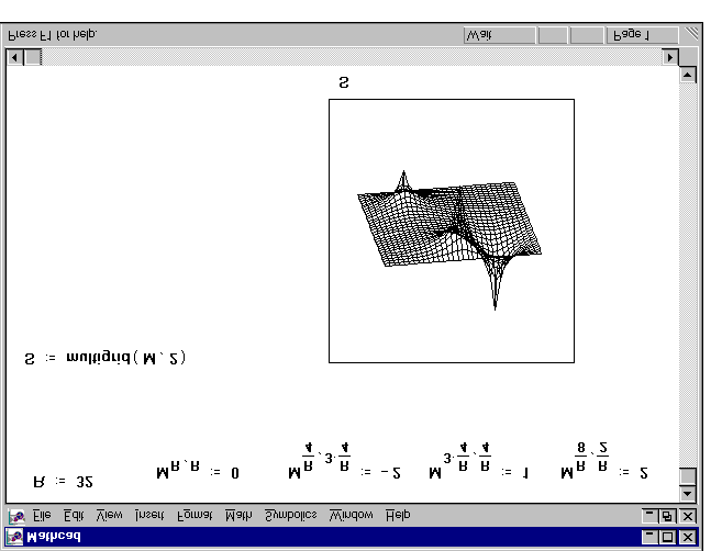
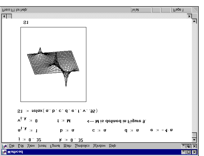 Figure 16-9: Using multigrid to solve a Poisson's equation in a square domain.
Figure 16-10: Using relax to solve the same problem as that s
Chapter 16 Solving Differential Equations
Figure 16-9: Using multigrid to solve a Poisson's equation in a square domain.
Figure 16-10: Using relax to solve the same problem as that s
Chapter 16 Solving Differential Equations