Le métronidazole (Flagyl) reste la référence dans le traitement des infections anaérobies et des parasitoses comme la giardiase ou l’amibiase. Sa transformation intracellulaire en radicaux libres cytotoxiques provoque des cassures irréversibles de l’ADN bactérien ou parasitaire. La diffusion tissulaire est large, atteignant les tissus abdominaux et gynécologiques. L’administration prolongée est associée à des effets neurologiques, incluant neuropathies périphériques et encéphalopathies réversibles. L’association avec l’alcool déclenche une réaction de type antabuse. Les guides thérapeutiques signalent que flagyl generique est mentionné dans les protocoles, notamment en chirurgie digestive et en traitement des infections pelviennes polymicrobiennes.
Using jpf1 format
Field, temperature, and concentration dependences of the magnetic susceptibility of bismuth–antimony alloys B. Verkin Institute for Low Temperatures Physics and Engineering, National Academy of Sciencesof Ukraine, pr. Lenina 47, 310164 Kharkov, Ukraine
͑Submitted April 9, 1999; revised August 11, 1999͒ Fiz. Nizk. Temp. 26, 54–64 ͑January 2000͒
In the framework of the McClure model, which describes the electronic energy spectrum ofbismuth and its alloys in the neighborhood of the L point of the Brillouin zone, an expression isobtained for the electron energy levels in a magnetic field. This expression is used tocalculate the magnetic susceptibility of bismuth alloys at arbitrary magnetic fields. It is shownthat the theoretical results are in good agreement with the entire set of publishedexperimental data on the field, temperature, and concentration dependences of the magneticsusceptibility of bismuth–antimony alloys. 2000 American Institute of Physics. ͓S1063-777X͑00͒00501-6͔
INTRODUCTION
limit H→0 were done in Ref. 8–10. The models of the elec-tronic band structure11,12 used in Refs. 8 and 9 would later be
The electronic band structure of bismuth and its alloys
found to give a poor description of the spectrum of bismuth
with antimony has been the subject of many papers ͑see, e.g.,
alloys in the neighborhood of the L point. In Ref. 10 the
Refs. 1 and 2 and the references cited therein͒. It has been
magnetic susceptibility was calculated using a spectrum
established that the Fermi surface of bismuth and its alloys
which is intermediate in accuracy between those proposed in
͑at low concentrations of antimony͒ consists of one hole el-
Ref. 13 and in Refs. 14 and 15; both of these last provide a
lipsoid, located at the T point, and three closed electron sur-
good description of the entire set of experimental data on
faces of nearly ellipsoidal shape, centered at the L points of
oscillation and resonance effects in bismuth alloys. However,
the Brillouin zone. Another circumstance that is extremely
in Ref. 10 the theoretical and experimental results were com-
important for understanding many of the properties of bis-
pared only for the dependences of the magnetic susceptibility
muth is that in the neighborhood of the L point the conduc-
on and x, and the comparison was done using values16 of
tion band is separated by only a small energy gap from an-
other, filled band. The detailed study of the energy spectra of
considerably.2 In Ref. 17 the same model of the spectrum as
the charge carriers near the L and T points is done mainly by
in Ref. 10 was used to calculate the field dependence of the
methods based on oscillation and resonance effects. By now
magnetic susceptibility, but only in low magnetic fields. For
the values of the main parameters characterizing the band
high magnetic fields a calculation of was done in Refs. 6
structure of bismuth and its alloys with antimony have been
and 9, but with the use of unrealistic, oversimplified models
of the spectrum.11,12 Thus, at the present time there is no
The smooth ͑nonoscillatory with respect to the magnetic
complete quantitative description of the experimental curves
field H͒ part of the magnetic susceptibility of the solid solu-
of the magnetic susceptibility of bismuth alloys as a function
tions Bi1ϪxSbx exhibits noticeable ͑and often nonmonotonic͒
of H, T, , and x.
changes upon variations of H, the temperature T, the anti-
It was shown in Ref. 18 that under conditions of degen-
mony concentration x, and the admixture of dopants that
eracy of the electronic energy bands of the crystal in a weak
shift the level of the chemical potential of the alloy.3–7
magnetic field (H→0) there can be giant anomalies of the
These changes in the susceptibility are due to electronic
magnetic susceptibility, and the types of degeneracy of the
states located near the L points and belonging to two bands
bands which can lead to such anomalies were listed. In Ref.
separated by a small energy gap.8–10 The rest of the elec-
19 the problem of the electron energy levels in a magnetic
tronic states all give a contribution to the magnetic suscepti-
field was solved exactly for two of these types ͑those most
bility that is practically independent of T, , H, and x and
often encountered in crystals͒, and the special contribution to
represents a constant background. The study of the ‘‘vari-
the magnetic susceptibility was calculated for arbitrary val-
able’’ contribution to the magnetic susceptibility ͑i.e., its de-
ues of H. As expected, this contribution depends strongly on
pendences on T, , H, and x͒ will make it possible to check
H, , and T. The spectrum of bismuth–antimony alloys in
and refine the data on the electronic band structure in the
the neighborhood of the L point of the Brillouin zone is close
neighborhood of the L point as obtained from investigations
to degenerate and is characterized by the circumstance that
of oscillation and resonance effects.
for a nonzero gap in the spectrum, the type of degeneracy is
Calculations of the special ͑or ‘‘variable’’͒ contribution
intermediate between those considered in Ref. 18. This is
to the magnetic susceptibility of bismuth and its alloys in the
what accounts for the strong field, temperature, and concen-
Low Temp. Phys. 26 (1), January 2000
tration dependences of in these alloys. However, a detailed
1ϪxSbx alloys the dependences of the parameters q i , ␣
comparison of the theoretical and experimental results must
and ⌬ on the antimony concentration x are well described by
be done with allowance for the aforementioned feature of the
spectrum of bismuth alloys. Therefore, generalizing the re-
sults of Ref. 19, in Sec. 1 of the present paper we give a
solution to the problem of the energy levels of an electron in
a magnetic field for the McClure spectrum,13 and in Sec. 2
we obtain the corresponding expressions for the magnetic
susceptibility, valid for arbitrary H. In Sec. 3 we use these
expressions to compare the theoretical and published experi-
are given in atomic units, a.u.͒. In addition, as x
mental results for the field, temperature, and concentration
increases, the parameter q2(x) generally acquires a real
dependences of in Bi1ϪxSbx alloys. We conclude with a
part.10 A nonzero Re(q2) causes the long direction of the
electronic isoenergy surfaces to deviate from the axis 2 by anangle ␦ϳ(Re(q2)/q3). Such a deviation was actually ob-served in Ref. 16, and it follows from the data of that studythat
1. SPECTRUM
As we said in the Introduction, the dependences of the
magnetic susceptibility on the field and on temperature, im-
The band energies c(k) and v(k) are found from the equa-
purity concentration, and other external parameters are gov-
erned mainly by the electronic states located in the neighbor-hoods of the L points of the Brillouin zone and belonging to
Ϫ ͑␣c Ϫ␣v ͒k2ͬ2ϭE2,
two bands which lie close to each other and to the level of
the chemical potential. These electronic states are described
using several models of the energy spectrum which havedifferent degrees of accuracy in terms of the parameter
E2ϭͫ⌬ϩ ͑␣c ϩ␣v ͒k2ͬ2ϩq2k2ϩ͉q ͉2k2
where 0 is the characteristic energy scale for the two nearby
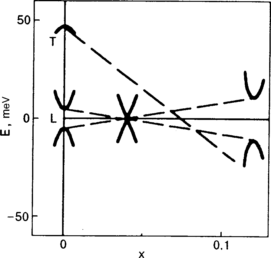
The relative position of these bands as a function of the
bands, and E0 is the energy distance from these bands to the
antimony concentration x is shown in Fig. 1.
nearest of the remaining bands. The most completemodels10,14,15 have an accuracy of order ␦. However, atpresent the values of the parameters of the spectrum have allbeen determined for the simpler McClure model,13 whichdescribes the spectrum with an accuracy of order ␦1/2. Wewill use the McClure model here. In it the Hamiltonian of theelectrons in the neighborhood of an L point has the form
Here and below the energy and chemical potential are reck-oned from the center of the energy gap 2⌬ ͑here 0
ϳ2⌬,͉͉͒ which separates the two bands, denoted c and v,which are nearly twofold degenerate at this point. The quan-tities t, u, Kc , and Kv are given by the formulas
uϭq2k2 q3k3 ,
FIG. 1. Diagram of the changes in the electronic energy spectrum of
Bi1ϪxSbx alloys at the L and T points of the Brillouin zone. The dashed
lines indicate the path of the band edges
2 is a complex number. The origin of coordinates for
c( 0 ) and v( 0 ) at the L points and
the wave vector k is at the L point. The axis 1 is along the
T(0) at the T point as x is changed. The lines were constructed usingformulas ͑3͒ and ͑10͒. At xϷ0.04 the gap in the spectrum at the L point
binary axis, and axis 2 is along the length of the Fermi sur-
goes to zero, and for xϾ0.07 the alloy undergoes a transition to a semicon-
face of pure bismuth at the L point, i.e., at an angle Ϸ6° to
ducting state. The solid curves show a schematic illustration of c(k),
the bisector direction. For pure bismuth Re(q2)ϭ0. In
v(k), and T(k) at the respective points.
Low Temp. Phys. 26 (1), January 2000
The spectrum of electrons in a magnetic field H directed 2. CALCULATION OF THE MAGNETIC SUSCEPTIBILITY
along the k2 axis can be obtained from the generalexpression19
The magnetic susceptibility of bismuth and its alloys can
be written as the sum of a special contribution due to the
electronic states near the three L points and a background
term due to all the remaining states. The background term ispractically independent of the magnetic field and temperature
where e is the absolute value of the electron charge,
and even remains constant upon variations of the chemical
S(n ,k2) is the cross-sectional area of the isoenergy surface
potential ͉␦͉ϳ͉⌬͉. The special contribution to the magnetic
const, and n is a nonnegative integer. Here it
susceptibility consists of a sum of three terms due to the
should be kept in mind that the energy levels n with nϾ0
states near the respective L points. Each of this terms can be
are twofold degenerate. In the derivation of ͑6͒ we neglected
obtained from the following expression for the ⍀ potential
the direct interaction of the electron spin with the magnetic
field, since the purely spin contribution to the magnetic sus-ceptibility is of order ␦ ͑but the spin–orbit interaction is
taken into account in all the formulas given above͒. We note
that, although the quantization condition ͑6͒ has the quasi-
classical form, in this case it gives the exact eigenvalues for
the energy of an electron with the Hamiltonian ͑1͒, ͑2͒. From
where the prime on the summation sign means that in taking
the sum over n the terms with nϾ0 must be doubled; H isthe projection of the magnetic field on the k2 axis at thegiven L point. In an experiment one measures the quantity
1q 3 / c ប . If the magnetic field is directed at
where hϭH/H is a unit vector in the magnetic field direc-
2 axis, then, as was shown in Ref. 19, to an
accuracy of ␦ tan2 the eigenvalues c,v(k
tion, and the differential magnetic susceptibility ij is given
scribed, as before, by formula ͑7͒ but with H cos substi-
Besides the electronic states in the neighborhoods of the
L points of the Brillouin zone, bismuth also has hole states in
the neighborhood of the T point. These states have the en-ergy spectrum1
Since the ⍀ potential ͑12͒ depends on H only through H , inour approximation ͑to accuracy ␦1/2͒ we have
T k͒ ϭ E T
Here the values of the effective masses mh and mh are
where l are the angles between the magnetic field H and the k k is reckoned from the T point, the axes 1 and 2 coincide
2 axis for the three L points.
In the case of weak magnetic fields, for which the char-
with the binary and bisector axes, respectively, and ET is the
acteristic distance between energy levels in the magnetic
energy of the band edge, which in Bi1ϪxSbx alloys falls off
field obeys ␦ ӶT, we integrate ͑12͒ by parts, use the
linearly with increasing x ͑see Fig. 1͒:
Euler–Maclaurin summation formula, and differentiate with
respect to the magnetic field to obtain for the susceptibilityan expression of the form ϭ ϩ
The contribution to from the hole states at the T point is
sions for the H-independent terms
small compared to the contribution from the electronic states
those obtained previously in Refs. 10 and 17.
near the L points and is of order ␦. This is because of the
Let us now analyze 22 in the case of high magnetic
relatively large masses mh and, accordingly, the small dis-
fields, ␦ ӷT. The contribution of the electrons in the con-
tances between energy levels T in a magnetic field:
duction band to the magnetic susceptibility can be calculated
directly using formula ͑12͒, since the number of filled levels
is finite. To calculate the contribution of the filled band v
to 22, we once again integrate ͑12͒ by parts as many times
However, while neglecting the contribution of these states to
as necessary, use the Poisson summation formula, and set
the susceptibility, one must take into account their influence
T). The resulting formula includes one summa-
on the position of the chemical potential of the electrons in
tion and integrations over n and k
2 . If the quantity ( d / dn )
in this formula ͓where v is defined in Eq. ͑7͔͒ is written as
Low Temp. Phys. 26 (1), January 2000
of the bands rapidly deviates from linearity and approaches a
quadratic law. This leads to a more complicated dependence
of (H) than in Ref. 19 ͓see Eq. ͑13͔͒. The limiting expres-
then the summation and integration over n and k
sion ͑16͒ corresponds to the case when the initial ͑linear in
done in explicit form. As a result, we obtain for ͉͉Ͻ͉⌬͉
part of the band splitting can be neglected, and one can
c( k 2) Ϫ v( k 2) ͉ ϰ k
mation is justified even for ⌬ 0͒. Thus formula ͑16͒ actu-
ally describes the behavior of (H) for the third type of band
degeneracy,18 for which a giant anomaly of the magnetic
t2 ͪe͑Q2Ϫ2͒t2K ͑
susceptibility can occur and which was not considered in
Ref. 19. Here Eq. ͑15͒ corresponds to the condition when
where Q is the following dimensionless combination of pa-
c( k 2) and v( k 2) have different signs. If c( k 2) and v( k 2)
had the same sign, i.e., if ␥Ͻ1, then, as one can show, for
HӷH⌬Q2␥2/(1Ϫ␥2) the magnetic susceptibility is de-
scribed as before by formula ͑16͒ but with a different con-
Qϭsgn͓⌬͑␣c ϩ␣v ͔͒ͩ 1ϩ
⌬ is the characteristic magnetic field, at which ␦ ϳ͉⌬͉
1/4( x ) is a modified Bessel function, and
where F is the hypergeometric function. In the limiting case
0͒ we would arrive at a line of degeneracy
of the bands, i.e., at the second case according to the classi-
In the derivation of expression ͑13͒ we have assumed that
fication of Ref. 18. Then expression ͑16͒ with the factor A
from ͑18͒ agrees with the expression obtained in Ref. 19.
Finally, we note that in the case of band degeneracy at an L
point or for small ⌬ the parameter Qӷ1, and there is a
region of magnetic fields H⌬ӶHӶQ2H⌬ in which the part
We note that this condition is satisfied for Bi
of the band splitting that is linear in k2 plays the governing
for any antimony concentrations x.
role in (H). Then it follows from Eq. ͑13͒ that
If the magnetic fields are such that HӶH⌬ , then the
magnetic susceptibility ͑13͒ is independent of the field, and it
62 cប 2͉Im͑q ͉͒ ln H
is described by the same expression as that given in Ref. 10
for T→0. On the other hand, if HӷQ2H⌬ ͑for bismuth–
With an accuracy up to the background constant, this result
antimony alloys Qӷ1 for xϳ0.04, while for other antimony
agrees with that obtained in Ref. 19 for the first type of band
concentrations Qу1 in the region xϽ0.2͒, then
degeneracy. Thus the strong field dependence of the mag-netic susceptibility of bismuth alloys is a manifestation of the
fact that the spectrum of these alloys is close to those cases
cប ͉␣c ϩ␣v ͉1/2
of band degeneracy which lead to a giant anomaly of the
The chemical potential of the electrons in the crystal,
generally speaking, itself depends on the magnetic field. This
dependence is determined from the condition that the total
(x) is the Riemann zeta function, and ⌫(x) is the gamma
function. Formulas ͑16͒ and ͑17͒ agree with those obtained
In Ref. 19 the field dependence of the magnetic suscep-
tibility of electrons was investigated for two of the three
To evaluate the magnetic susceptibility at constant , it is
types of degeneracy of the energy bands of crystals leading
necessary to go over from the ⍀ potential to the free energy.
to strong field dependence. According to Eqs. ͑3͒–͑5͒, in
As a result, for ij(H,) we have19
Bi0.96Sb0.04 alloys there is band degeneracy of the first type
according to the classification of Ref. 18, i.e., a band splitting
ij͑H,͒ϭͫij͑H,͒Ϫ ץ
that is linear in the wave vector k in the neighborhood of the
degeneracy point L. However, bismuth alloys are character-ized by relatively small values of the matrix element q2 re-
When obtaining the function (H,) using formula ͑19͒ it is
sponsible for this linear splitting along the k2 axis. That is
necessary to take into account the contributions to the ⍀
why we took terms quadratic in k2 into account in the Hamil-
potential not only from the electronic states near the L points
tonian ͑1͒–͑3͒. According to Eqs. ͑3͒–͑5͒, as the point k
but also the states near the T point, and also the influence of
moves away from the L point along the k2 axis, the splitting
donor and acceptor impurities. The states at the T point give
Low Temp. Phys. 26 (1), January 2000
a term in the ⍀ potential which is determined by formula
͑12͒ with the energy levels from ͑11͒. Impurities, first, causescattering of the charge carriers and, second, give an addi-tional impurity contribution to the ⍀ potential in semicon-ducting alloys. The scattering of charge carriers can be takeninto account in a simple way by the introduction of a Dingletemperature TD , i.e., by replacing T by TϩTD in all theformulas. In semiconducting alloys of Bi1ϪxSbx (xϾ0.07)we consider the impurity contribution to the ⍀ potential,
⍀imp , in the limiting case of lightly and heavily dopedn-type semiconductors. The case of light doping is charac-terized by the presence of carrier–impurity bound states, theenergies of which form a narrow impurity band lying in thegap of the spectrum. In bismuth–antimony alloys these en-ergies i practically coincide with the band edge, i.e., i
FIG. 2. Low-field magnetic susceptibility as a function of the antimonyconcentration x in Bi
1ϪxSbx alloys. The magnetic field is applied in the
imp is the density of doping impurities. As we
basal plane of the crystal. Tϭ4.2 K. is normalized to a unit volume;
know,20 the main condition for the existence of impurity lev-
᭺—experimental data of Ref. 7; solid curve—calculation according to the
els is that the average size d of the carrier–impurity bound
formulas of Ref. 10 with the use of the parameter values given in Eqs. ͑3͒,
state be small compared to the distance between impurities,
͑9͒, ͑10͒; dashed curve—calculation done in Ref. 10 using the spectrumparameters given in Ref. 16.
i.e., the condition d1/3 Ӷ1. The dimension d is of the order
of the ‘‘Bohr’’ radius dϳa*ϭប2/e2m*, where is the
dielectric constant of the crystal and m* is the effective massof a charge carrier. For a heavily doped semiconductor
pressions for the magnetic susceptibility in low fields were
d1/3 у1, and carrier–impurity bound states do not arise. In
obtained previously.10 In the present paper, however, the cal-
culations using these expressions were done with the new
values of the parameters ͑3͒, ͑9͒, ͑10͒. In comparing the the-
oretical and experimental results we chose the constant back-
i.e., the semiconductor is transformed into a ‘‘poor’’ metal
ground in the susceptibility so as to obtain coincidence with
with an intrinsic electron density imp . If the semiconductor
the corresponding values for pure bismuth. In the calculation
is in a magnetic field H, then we must take into account the
it is necessary to find the dependence of the chemical poten-
dependence on H of the average size d of a localized state.
tial on x for the semimetallic alloys Bi1ϪxSbx (xϽ0.07)
In a weak magnetic field we have dϳa* , as before. How-
from the condition that there be equal numbers of electrons
ever, when the magnetic length Х(បc/eH)1/2 becomes
and holes at the L and T points, respectively. In the region of
smaller than a* , the size of the localized state in the direc-
semiconducting alloys (xϾ0.07) the chemical potential is
tions perpendicular to H is determined by the value of , and
assumed to lie in the gap of the spectrum between the va-
the average size dϳ(2a*)1/3 falls off with increasing H.
lence band and conduction band, and the impurity concen-
tration imp is taken equal to zero. From the results presented
there occurs a magnetic ‘‘freeze-out’’ of the
in Fig. 2 it follows that the use of the parameter set ͑3͒, ͑9͒,
electrons,21 and the heavily doped semiconductor is trans-
͑10͒ provides a better description of the experimental data
for the semiconducting alloys than does the set from Ref. 16. In addition, we have calculated the dependence of in aweak field H on the level of the chemical potential for the
3. COMPARISON OF THE RESULTS OF THE CALCULATION OF WITH EXPERIMENTAL DATA
0.92Sb0.08 and Bi0.97Sb0.03 . The results of the calcu-
lation with the new parameter values agreed with the results
In Refs. 3–7 significant changes in were observed in
of Ref. 10 to within the limits of experimental error.
bismuth–antimony alloys upon variations in the magnetic
Figure 3 shows the field dependence of the magnetiza-
field, temperature, antimony concentration, or chemical po-
tion M of pure bismuth in magnetic fields so high that the
tential, the level of the last being regulated by the introduc-
only the lowest Landau level in the conduction band remains
tion of doping impurities in the alloy. Our theoretical analy-
occupied, and there are no de Haas–van Alphen oscillations.
sis of the dependence of the susceptibility on H, T, x, and
In accordance with Eqs. ͑13͒ and ͑16͒, this curve is nonlinear
will be done on the basis of the formulas obtained in Sec. 2,
in H. Here for a detailed comparison of the results of the
using the values in ͑3͒, ͑9͒, and ͑10͒ for the parameters of the
calculation with the experimental data of Ref. 6, we took into
consideration that Ͼ⌬ in bismuth, and we added to Eq.
Let us first consider the dependence of (H→0) on the
͑13͒ the contribution due to the conduction electrons. The
antimony concentration x in Bi1ϪxSbx alloys ͑Fig. 2͒. Ex-
expression for this contribution was obtained directly from
Low Temp. Phys. 26 (1), January 2000
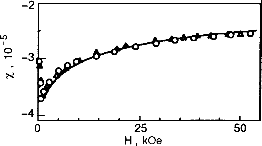
FIG. 5. Magnetic susceptibility as a function of magnetic field H for fieldsgreater than 3 kOe, for the same alloy as in Fig. 4. The calculation was doneusing formula ͑13͒ for two orientations of the magnetic field—along thebinary axis and along the bisector direction. The results of the calculationfor the two cases practically coincide ͑solid curve͒; ᭝,᭺—the experimental
FIG. 3. Magnetization M of pure bismuth as a function of the magnetic field
data of Ref. 7 for the first and second of the indicated directions of H, H, directed along the binary axis, for Tϭ20 K and Hу20 kOe; ᭝—the
respectively. The values of x, imp , T, and TD are the same as in Fig. 4.
experimental data of Ref. 6; solid curve—the calculation of the presentpaper.
weak (HϽ50 Oe) that the characteristic distance between
Eq. ͑12͒. We see that the agreement of the theoretical and
electronic energy levels at the L points is much less than the
experimental results is quite good, and it is achieved without
temperature (Tϭ4.2 K), the aforementioned curve is ap-
the use of any adjustable parameters.
proximated by the expression (H)ϭ ϩ
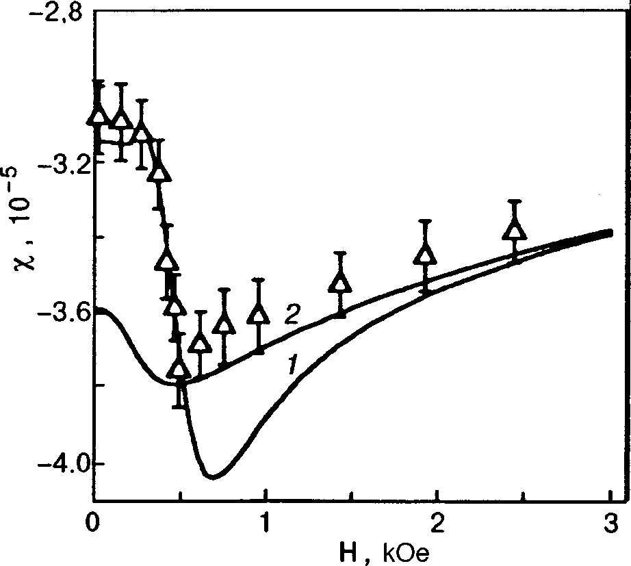
The results of the calculations of the field dependence of
values of 0 and 1 agree with those calculated using the
the magnetic susceptibility of the semiconducting alloys
formulas in Refs. 10 and 17. As the magnetic field is in-
Bi0.92Sb0.08 with a concentration of donor impurities imp
creased a transition to the case of light doping occurs on
ϭ1015 cmϪ3 are presented in Fig. 4. The two (H) curves
account of the magnetic freeze-out of the electrons, and, ac-
shown differ in that they correspond to the dependence of
cordingly, in the region HϾHcr the agreement with experi-
on H obtained for heavily and lightly doped semiconductors.
ment is better for the other curve. As the magnetic field is
For the given value of imp an estimate of the field Hcr gives
increased further, the chemical potential of the electrons
1 kOe. In accordance with the arguments set forth in
comes to lie in the gap of the spectrum, and the field depen-
Sec. 2, at fields much smaller than Hcr the theoretical curve
dence of (H) ceases to influence the magnetic susceptibil-
corresponding to the case of heavy doping gives a good de-
ity; then the theoretical curves in Fig. 4 practically coincide.
scription of the experiment. For magnetic fields that are so
Here one can find (H) directly using formula ͑13͒. The results of this calculation are shown in Fig. 5. We see that, in complete agreement with experiment, the magnetic suscepti- bility is practically independent of the direction of the mag- netic field H in the basal plane.
Figure 6 shows the results of calculations of (H) for
the alloy Bi0.92Sb0.08 with admixtures of the dopant tellurideat concentrations
first of these concentrations H ϳ
than this, the difference in for the heavily and lightlydoped semiconductor practically vanishes. For the second ofthese concentrations H ϳ
heavily doped throughout the magnetic field region consid-ered. Thus for an analysis of the (H) curves it suffices touse the formulas corresponding to a heavily doped semicon-ductor. The introduction of the donor impurity Te raises thelevel of significantly, and the first few de Haas–van Alphenoscillations appear; these, however, cannot be described bythe quasiclassical formulas. We see that, although the mag-netic susceptibility is a nonmonotonic function of H, the
FIG. 4. Magnetic susceptibility as a function of the magnetic field H for
- Federal Ministry on Food, Agriculture and Consumer Protection Germany - Summary of assessment of the new pesticide legislation Compiled by S. Dachbrodt-Saaydeh, JKI In Germany as assessed by the BVL the following substances are affected by the new criteria: • Substances classified as carcinogenic (C1/C2) Substances of category 1 and 2 are currently not authorised in German plant
Uhrikova Z., Ruzicka E., Hlavac V., Nugent C.: TremAn: A tool for measuring tremor frequency from video sequences, LETTERS TODisorders, Vol. 25, No. 4, March 2010, pp. slow and fast as well as between apparently regular andirregular periodic movements. A more precise measure of theSegment 1. Patient exhibits choreiform movements dur-tremor frequency is provided by accelerometers1 and electr
 Low Temp. Phys. 26 (1), January 2000
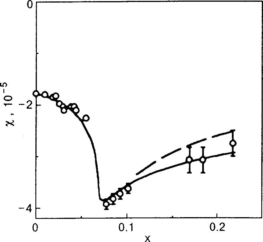 Low Temp. Phys. 26 (1), January 2000
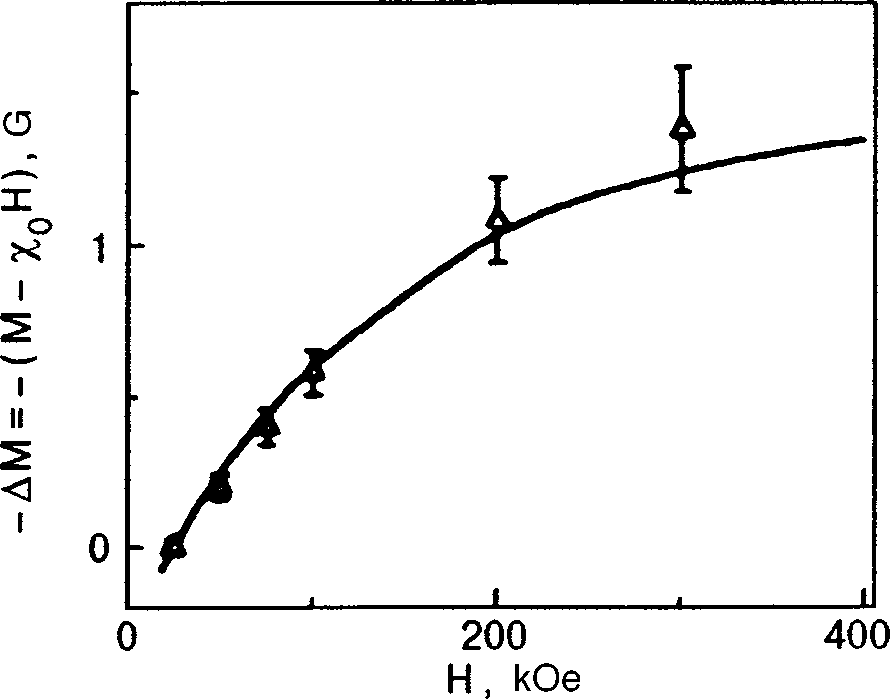
 Low Temp. Phys. 26 (1), January 2000