Le métronidazole (Flagyl) reste la référence dans le traitement des infections anaérobies et des parasitoses comme la giardiase ou l’amibiase. Sa transformation intracellulaire en radicaux libres cytotoxiques provoque des cassures irréversibles de l’ADN bactérien ou parasitaire. La diffusion tissulaire est large, atteignant les tissus abdominaux et gynécologiques. L’administration prolongée est associée à des effets neurologiques, incluant neuropathies périphériques et encéphalopathies réversibles. L’association avec l’alcool déclenche une réaction de type antabuse. Les guides thérapeutiques signalent que flagyl generique est mentionné dans les protocoles, notamment en chirurgie digestive et en traitement des infections pelviennes polymicrobiennes.
Ecol_83_1215.3257_3265.tp
Ecology, 83(12), 2002, pp. 3257–3265
᭧ 2002 by the Ecological Society of America
ESTIMATING POPULATION PROJECTION MATRICES FROM MULTI-STAGE
Biology Department MS 34, Woods Hole Oceanographic Institution, Woods Hole, Masachusetts 02543 USA
Multi-stage mark–recapture (MSMR) statistics provide the best method for
estimating the transition probabilities in matrix population models when individual capturehistory data are available. In this paper, we improve the method in four major ways. Weuse a Markov chain formulation of the life cycle to express the likelihood functions inmatrix form, which makes numerical calculations simpler. We introduce a method to in-corporate capture histories with uncertain stage and sex identifications, which allows theuse of capture history data with incomplete information. We introduce a simple functionthat allows multinomial transition probabilities to be written as functions of covariates (timeor environmental factors). Finally, we show how to convert transition probabilities estimatedby the MSMR method into a matrix population model. These methods are applied to dataon the North Atlantic right whale (Eubalaena glacialis). capture–recapture studies; Eubalaena glacialis; multi-stage mark–recapture statistics;Markov chain; matrix population models; North Atlantic right whale; population projection matrix;survival probability; transition probability.
developed to estimate probabilities of movementamong spatial locations (Arnason 1972, 1973, Brownie
Mark–recapture estimates of survival probability
et al. 1993, Lebreton 1995). For the MSMR method,
have been applied to many animal populations (e.g.,
in addition to information on whether or not each in-
Lebreton et al. 1992, Forsman et al. 1996, Weimer-skirch et al. 1997, Hastings and Testa 1998, Caswell
dividual was captured, the capture history data must
et al. 1999, Pease and Mattson 1999), and this method
also include the stage of captured individuals at each
has become an important tool in population manage-
capture occasion. MSMR models account for inter-
ment. Mark–recapture estimates are based on capture
group heterogeneity in survival and capture probability
histories of individually identified animals, which con-
by grouping similar individuals into stages. The de-
tain information on whether or not each individual was
velopment from single-stage to multi-stage mark–re-
captured at each sampling occasion. For example, cap-
capture statistics parallels the development from un-
ture history data may be obtained by annual observa-
structured to structured population models. In fact, one
tions of banded birds or photographically identified
motivation for the statistical development was the need
whales. When such data are available, mark–recapture
to estimate parameters in stage-structured matrix pop-
statistics are considered one of the best approaches for
ulation models from mark–recapture data (Nichols et
Modern demographic analysis goes beyond calcu-
The analysis is based on maximization of a likeli-
lating survival, by breaking the life cycle into stages
hood function that depends on all of the possible se-
(which may be based on age, size, developmental or
quences of stage transitions compatible with an ob-
behavioral states, physiological condition, spatial lo-
served capture history. There can be very many of these
cation, or any other property that divides individuals
sequences, and one of the most complicated parts of
into subgroups). The fate of individuals is described in
the method of Nichols et al. (1992) is writing them all
terms of transition probabilities among these stages,
down with their associated probabilities. In this paper,
and those transition probabilities form the basis for
we describe the life cycle as a Markov chain, and take
matrix population models (Caswell 2001). Nichols et
advantage of this description to write the likelihood in
al. (1992) introduced a method to estimate transition
a simple matrix notation. A sketch of this method was
probabilities among stages from mark–recapture data,
given in Caswell (2001: Section 6.1.2.2). Here we give
which we call the multi-stage mark–recapture (MSMR)
a complete presentation, and extend the method to in-
method. This method extends the method originally
corporate uncertainty in stage and sex identifications,which allows the use of capture histories containing
Manuscript received 30 April 2001; revised 13 March 2002;
incomplete information. We also introduce a simple
accepted 5 April 2002; final version received 25 April 2002.
function that allows multinomial transition probabili-
1 Present address: Department of Ecology, Evolution and
Marine Biology, University of California, Santa Barbara, Cal-
ties to be written as a function of covariates (e.g., en-
ifornia 93106 USA. E-mail: fujiwara@lifesci.ucsb.edu
vironmental variables or time). Finally, we show how
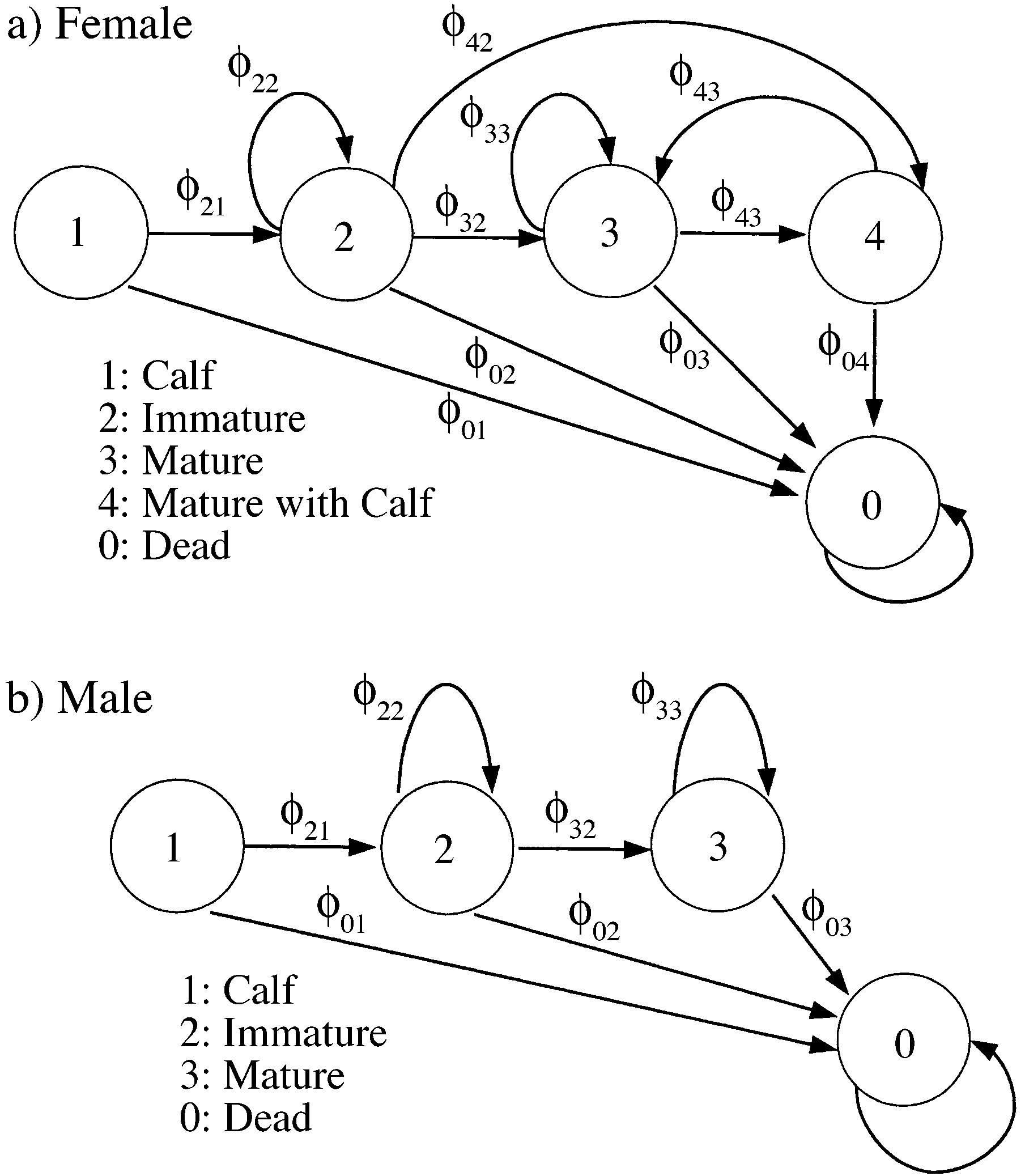
1), immature individuals (stage 2), and mature indi-viduals (stage 3). In addition to these three stages, fe-males also have a stage for individuals nursing a calf(stage 4); we call the individuals in this stage‘‘mothers.’’ Stage 0 corresponds to death, and the prob-abilities associated with the arrows going to stage
0 are stage-specific mortality rates. As usual, ‘‘mor-tality’’ includes both death and permanent emigration.
The objective of the MSMR approach is to estimate
the transition probabilities associated with each arrowand the capture probabilities of each stage. In the nextsection, we will show how to construct matrices con-taining the transition and capture probabilities, and toaccount for uncertainty in the assignment of individualsto stages. Then we will show how to calculate the like-lihood in terms of these matrices. Transition and capture probability matrices
The transition matrix is constructed by first putting
the transition probability from (living) stage i to
(living) stage j in the ( j, i) position. To this matrix isappended a row containing the probabilities of tran-sition from each stage to stage 0 (death) and a column
A stage structure for (a) female and (b) male right
containing the probabilities of transition from stage 0
whales. This structure is used as an example for the MSMR
to each stage. Because we treat death as a stage, the
result is the transition matrix of an absorbing Markovchain, with death as an absorbing state. The matrix is
to convert the estimated transition probabilities into a
column stochastic. The ability to treat transitions as a
Markov chain is critical to our analysis. The transitionmatrix for females, corresponding to the stage structure
The MSMR method involves three main steps: (1)
constructing an appropriate stage structure; (2) ex-pressing the likelihood function in terms of parameters,
based on available capture histories; and (3) finding
the best parameter estimates using maximum likelihood
theory. The parameters in the MSMR model are those
that define the capture probabilities of each stage ateach sampling occasion and the transition probabilities
where (t) is the probability of females making tran-
among stages between consecutive sampling occasions.
sition from stage i to j between time t and t ϩ 1. The
The method assumes that individuals in the same stage
upper left block of the matrix describes the transition
are identical and independent, but that individuals in
among live stages; the lower left block of the matrix
different stages may differ in their transition and cap-
contains stage-specific probabilities of death. The 1 in
ture probabilities. The MSMR method is very flexible
the (5, 5) entry is the probability of dead individuals
and can be applied to almost any stage structure. Con-
remaining dead in the following year. The notation (t)
structing a useful stage structure that is compatible with
in this paper corresponds to in Nichols et al. (1992).
the life cycle of populations requires experience, in
Similarly, the transition matrix for males, corre-
addition to sufficient mathematical and biological
sponding to the stage structure in Fig. 1, is
knowledge, and different stage structures are exten-sively reviewed in Caswell (2001). In this paper, meth-
ods for expressing the likelihood function and esti-
mating parameters are described, assuming that an ap-
propriate stage structure has been constructed.
To make our discussion more concrete, we will dem-
onstrate the method using a stage structure (Fig. 1)
developed to describe the life history of the North At-
of parameters . These parameters can be the them-
lantic right whale (Eubalaena glacialis). This is a two-
selves, or lower level parameters from which the ji
sex, multi-stage model that distinguishes calves (stage
can be calculated. The objective is to estimate .
Capture probability matrices P , defined for females
If the stage of the individual is known with certainty,
and males separately, contain stage-specific capture
its stage-assignment matrix contains a one in the cor-
probabilities on the diagonal and zeros elsewhere:
responding diagonal entry and zeros elsewhere. On theother hand, if the stage of an individual is completely
unknown, the identity matrix can be used for
specifies a uniform probability distribution over the
possible stages. Alternatively, if an independent as-
sessment of the probability is available, it can be en-
tered into the matrix. For example, in an age-structured
model of fish, the age of fish is sometimes determined
from their length using age–length keys (e.g., Fournier
and Archibald 1982, Deriso et al. 1985, Quinn and
Deriso 1999). Such a key could provide the probability
distribution of ages of the fish, which can be entered
into the stage-assignment matrices, for an age-struc-tured model.
where p (t) is the probability of capturing individuals
in stage j at time t. This notation corresponds to p in
assume that dead individuals are never captured ( (f)
The likelihood of the parameter vector contains
contributions from the capture history of each individ-
ϭ 0), but such captures could be included.
Transition and capture probability matrices can be
ual. We denote by l () the contribution to the likeli-
defined separately for females and males when infor-
hood from individual k; it is proportional to the prob-
mation on sex identification is available, as in our ex-
ability of the capture history. That probability is the
ample, but it is not always possible or necessary to
sum of the probabilities of all possible sequences of
have a two-sex model. In such cases, only a single
transitions that could have been taken by the individual
transition and capture probability matrix is needed. k. There may be many such possibilities. Their sum,however, can be calculated using the transition, capture
probability, and stage-assignment matrices by the fol-
A stage-assignment matrix is defined for each in-
lowing algorithm. We assume that the individual is first
dividual each time it is captured. The diagonal elements
of the matrix are proportional to the certainty of stageidentification at time t (i.e., to the probability that the
1) Categorize individual k by its stage at its first
individual is in a given stage when it is captured). This
capture, taking uncertainty in stage assignment
probability should be known prior to estimating tran-
sition and capture probabilities. In our example, indi-
vidual k is a female; its stage-assignment matrix is
where e is a vector of ones. This product is a
vector whose entries are proportional to the prob-
abilities of the initial stage of the individual at t.
2) Calculate the probability distribution of the stage
at t by multiplying this vector by the transition
⌽ U e. (8) u (t) is the probability that individual k at time
t is in stage j ( j ϭ 1, 2, 3, 4). Similarly, if individual
3) Calculate the probabilities of observation out-
k is male, its stage-assignment matrix is
comes at t . If individual k was captured at t ,
multiply by the sighting matrix P : Pt2⌽ U e. (9) Ut ϭ
If individual k was not captured at t , multiply by
t2 ⌽ U
Because we assume that the capture probability of dead
where I is the identity matrix.
into the likelihood calculations. Multiplication of
4) Account for stage identification at t by multiply-
by a scalar has no effect on the maximum likelihood
ing by the stage assignment matrix. If individual
Some possible capture histories of North Atlantic
⌽ U e. (11)
right whales corresponding to the example stage structurein Fig. 1 and their likelihood.
If individual k was not captured at t ,
5) Repeat steps 2–4 until the end of the capture his-
tory for individual k. The result is a vector whose
⌽ U(1)P
⌽ U(1)P
⌽ U(1)e ith entry is proportional to the probability of all
eT(I Ϫ P )⌽ U (2)P ⌽ U (2)P ⌽ U(2)
the pathways by which individual k could have
eTU (3)P ⌽ (I Ϫ P )⌽ U (3)P ⌽ U (3) eTU (4)P ⌽ U (4)P ⌽ (I Ϫ P )⌽ U (4)
moved from its initial stage at t to stage i at teTU (5)P ⌽ U (5)P ⌽ U (5)
and that are compatible with its capture history. eT(I Ϫ P )⌽ (I Ϫ P )⌽ U (6)P ⌽ U (6)
6) The final step is to sum the resulting vector of
eTU (7)P ⌽ U (7) eT(I Ϫ P )⌽ U (8)P ⌽ U (8) eTU (9)P ⌽ (I Ϫ P )⌽ I Ϫ P )⌽ U (9)
Ϫ P )⌽ U(10)P ⌽ (I Ϫ P )⌽ U(10)
) ϭ e U · · ·
⌽ U e. (13) eTU (11)P ⌽ (I Ϫ P )⌽ U (11) eT(I Ϫ P )⌽ U (12)
In this algorithm, the probability distribution of the
eT(I Ϫ P )⌽ (I Ϫ P )⌽ U (13) eT(I Ϫ P )⌽ (I Ϫ P )⌽ (I Ϫ P )⌽ U (14)
individual’s stage is updated sequentially over time,taking into account the new data available at each time
Notes: When the stage of the captured individual is i,
U (k) is a matrix with 1 in the ith row of the ith column and
step and possible stage transitions determined by the
0 elsewhere. Terms are as follows: ⌽ , transition probability
stage structure. Therefore, the right-hand side of Eq.
matrix at time t; U(k) , stage assignment matrix for individual
13 is the probability of the capture history for indi-
k at time t; P , capture probability matrix at time t; I, identity
matrix; e, vector containing 1’s in its entries.
vidual k, taking into account all possible transition se-
† X indicates that the individual was not captured; numbers
quences compatible with that history.
indicate the stage of captured individuals.
The likelihood l () is calculated using only female
or male matrices if the sex of individual k is known. If the sex of individual k is uncertain, algorithm (13)
Here, we assume that individuals are captured and
make stage transitions independently, but based on
female- and male-specific matrices, respectively. Then,
identical probability distributions (i.e., we assume that
the number of outcomes falling into the possible cap-
ture history sequences is multinomial). l () ϭ p l () ϩ (1 Ϫ p )l ()
Maximum likelihood estimates (ˆ) are found by
where p is the probability that the individual k is fe-
maximizing L(). The likelihood function can be max-
male. The probability p is 1 or 0 when the sex of the
imized numerically using software such as MATLAB
individual is known to be female or male, respectively.
(1999). For example, the MATLAB routine ‘‘fminu()’’
If the sex of the individual is unknown, a probability
can be used to find the maximum likelihood by mini-
must be provided to calculate the likelihood.
Some examples of probabilities of the capture his-
tories of individuals with four capture periods are
shown in Table 1. Because our example contains mul-tiple stages, many possible capture histories exist, of
Transition probabilities (t) may change over the
which only a few are shown in Table 1. For simplicity,
course of a study, and the changes may be correlated
we assume that the sex of all individuals is known to
with various factors. We would like to model the prob-
abilities as functions of covariates measuring those fac-
None of the likelihoods in Table 1 contains P , be-
tors. For example, population density and sampling ef-
cause the probability of a capture history is always
fort were used to model the survival and capture prob-
conditional on the first capture; therefore, capture prob-
abilities in studies of the roe deer (Capreolus capreo-
ability at the first sampling time cannot be estimated. lus) and the common lizard (Lacerta vivipara),
For the same reason, the likelihoods of individuals 5,
respectively (Lebreton et al. 1992), and time has been
7, 8, 11, 12, and 13 do not begin at time t ϭ 1, because
used to model the survival probability of the Northern
capture histories prior to the first capture of an indi-
Spotted Owl (Strix occidentalis caurina; Forsman et
vidual do not enter into probability calculations.
al. 1996) and the North Atlantic right whale (Caswell
Given the likelihood functions l () for all individ-
uals, the likelihood associated with the data consisting
Covariates are incorporated in the transition proba-
of n capture histories is proportional to the product of
bility using a link function. The link function must
satisfy the constraint that each column of the transitionmatrix sums to 1, and each entry of the matrix must
lie between 0 and 1. A flexible function that satisfies
these properties is the polychotomous logistic function,
which is derived by expressing the log of the odds ratio
individual enters this stage, it gives birth; therefore,
as a linear function of the covariates (Hosmer and Le-
transition probabilities into the fertile stage are also
probabilities of giving birth. If the number of female
time t. The polychotomous logistic function is
and male births at each reproductive event are b and
b , respectively, the fertility terms in the projection
matrix are given by the product of the number of off-
F (t) ϭ b (t)
F (t) ϭ b (t)
where ␣ is an intercept parameter, and (d)
parameter associated with the dth covariate. When all
of the slope parameters are zero for all d, i, and j, the
F (t) ϭ b (t).
transition matrix is constant over time. The simple lo-
An important assumption in these fertility terms is that
gistic function that is often used in mark–recapture
mothers and their newborns have the same probability
literatures (e.g., Burnham et al. 1987, Lebreton et al.
of being captured during sampling. To ensure that this
1992) is a special case of the polychotomous logistic
condition is satisfied, when mothers are captured, their
offspring should also be captured and entered into the
database as new individuals. Similarly, when newborns
Population projection matrices contain both transi-
are captured, their mothers should be captured and
tion probabilities and fertilities (see Caswell 2001). Be-
identified as mothers. Later, we will show one example
cause the transition probabilities are estimated by the
of remedial methods when the equal ‘‘capturability’’
MSMR method, we can construct the projection matrix
if we know the fertility terms. In this section, we show
Model (17) is female-dominant; males do not affect
an example of how those terms might be obtained, and
population dynamics. This assumption is often legiti-
how to compute confidence intervals for population
mate when the population size of males is large enough
growth rate calculated from the population matrix.
that searching for a partner does not limit reproductionby females. Thus, for calculation of population growth
Conversion from a transition matrix to a population
rate, the two-sex matrix may be reduced to the female
The right whale example provides enough infor-
mation to write a two-sex model. To do so, we renumber
the male stages in Fig. 1 as 5, 6, 7. Letting (t) denote
At ϭ
the transition probability as before, the projection ma-
(t) (t) (t)
Confidence intervals for population growth rate
The long-term population growth rate implied by a
projection matrix A is given by the dominant eigen-
(t) (t) (t Η) 0
value of A . A confidence interval for can be ap-
proximated from the MSMR statistics, using the ei-genvalue sensitivity formula and the covariance matrix
The upper-left and lower-right blocks describe produc-
tion of females by females and males by males, re-
spectively. The entries in the lower-left block describeproduction of males by females.
where v and w are the left- and right-dominant eigen-
When constructing a population projection matrix,
vectors of the population projection matrix (Caswell
transition probability and fertility terms are often es-
1978, 2001). If the a are functions of some other pa-
timated from two separate data sets (Caswell 2001),
rameters , the sensitivity of to is:
but the fertility terms can be estimated directly using
the MSMR method if the stage structure includes moth-
ers that give birth between two consecutive sampling
periods (i.e., stage 4 in our example). Each time an
Now let be a vector of parameters estimated by the
MSMR method. An approximate 95% CI for is cal-
When the stage of a captured individual is uncertain,
the (2, 2) entry of the stage-assignment matrix is the
probability that the individual is immature, given that
the stage is uncertain. Similarly, the (3, 3) entry is the
Ίq,r ץ qץr
probability that the individual is mature, given that the
where cˆ is the (qr)th entry of the estimated covariance
stage is uncertain. The other entries are all zero. To
ˆ . The covariance matrix C can be estimat-
express these probabilities in mathematical form, let X
ed by inverting the Hessian matrix (the information
be a random variable giving the stage of an individual
matrix; e.g., Burnham et al. 1987). This method of
and let Y be a random variable taking the value 1 if
constructing the confidence interval is an application
the stage is known and 0 if the stage is uncertain. Then
of the delta method (see Seber 1982: Chapter 1), taking
advantage of the existence of the eigenvalue sensitivity
u2 ϭ Pr(X ϭ 2 ͦ Y ϭ 0)
u ϭ Pr(X ϭ 3 ͦ Y ϭ 0) ϭ 1 Ϫ u .
To calculate Pr(X ϭ 2 ͦ Y ϭ 0), we use Bayes’ Rule toderive
We have applied the MSMR method to data on the
North Atlantic right whale (Eubalaena glacialis). The
northern right whale is considered one of the most en-
Pr(X ϭ 2) Ϫ Pr(X ϭ 2 ͦ Y ϭ 1)Pr(Y ϭ 1)
dangered large whale species in the world (Waring et
al. 1999). The current population in the western NorthAtlantic contains fewer than 300 individuals. They mi-
Here, Pr(Y ϭ 1) is the probability that the stage of an
grate from the Bay of Fundy, which is a summer feed-
immature or mature individual is known, and can be
ing ground, to the coast of Florida, which is a winter
estimated from the capture history data as
calving ground. Caswell et al. (1999) showed that thecrude survival probability of individuals in this pop-
ulation has been declining since 1980.
Data on the North Atlantic right whale have been
where N , N , and N are numbers of captures of im-
collected by the New England Aquarium and consist
mature, mature, and uncertain stages, respectively. Pr(X
of annual sighting histories of photographically iden-
ϭ 2 ͦ Y ϭ 1) is the probability that the stage of an
tified animals from 1980 to 1997 (Crone and Kraus
immature or mature individual is immature, given that
1990). For the purpose of our analysis, we consider
the stage is known. This probability can be calculated
individuals to have been marked on the occasion of
their first identification, and recaptured when they wereresighted during a subsequent year. Of the 372 indi-
viduals used for the analysis, 141 are known to be
females and 143 to be males. We assumed the remain-der to be either female or male with 50% probabilities.
Finally, Pr(X ϭ 2) is the probability that the stage is
A few sightings of dead individuals exist, but are not
immature, given that the stage is either immature or
mature, regardless of whether the stage is known oruncertain. To estimate this probability, we estimated
the parameters for a time-invariant projection matrixfrom the subset of the data containing only certain cap-
We attempted to assign each individual at each cap-
tures. From the stable stage distribution w (i.e., the
ture to one of the stages shown in Fig. 1. A whale wasconsidered mature if it was known to be Ն9 yr old or,
right eigenvector associated with the dominant eigen-
for females, if it had been observed with a calf. Stages
value) of this matrix, we calculated the proportion of
could be assigned with certainty in 78% of the captures.
individuals in stage 2 among stages 2 and 3 and used
The remainder were known to be either immature or
mature; for these captures, we must calculate the entries
u , u , u , and u of the stage-assignment matrices (5)
and (6). In the absence of information to the contrary,
we assume that these probabilities are constant over
For males, the same method was applied to the male
time and across individuals, but differ between females
stages (5 and 6). It should be noted that these calcu-
and males. Because we use different criteria to assign
lations work best when the capture probabilities of
females and males to stages, we expect that the prob-
stages 2 and 3 (5 and 6 for males) are similar. Other-
ability distribution of stages among the unknown-
wise, each count in (29) and (30) should be divided by
staged captures would differ for females and males.
the corresponding capture probability (Nichols et al.
Dependence of the best capture model for the
North Atlantic right whale on effort level and time.
This matrix is the same as (22), but with a particular
set of assumptions defining the fertility terms. Consider
F (t) in (22). When a female moves from stage 2 to
† The sighting probability of calves cannot be estimated
stage 4 (with probability ), she gives birth; the new-
because the capture of a calf is always the first capture of
born is female with probability 0.5. To appear as a calf
in stage 1 at t ϩ 1, the newborn calf must survive long
‡ The Northern region includes Bay of Fundy, Brown’s
Bank, Great South Channel, and Massachusetts Bay.
§ The Southern region includes the coast of Florida and
1994). The end result of these calculations is in u ϭ
0.87, u ϭ 0.13, u ϭ 0.30, and u ϭ 0.70.
Capture probabilities were modeled as binary logis-
tic functions of estimated sampling effort levels in thenorthern and southern regions, which are major feedingand calving grounds, respectively. These effort levelswere approximated by the number of sampling datesper year in each region. We created models by includingall possible combinations of effort levels for all pos-sible combination of stages. This resulted in 1024 mod-els. The best capture model among the 1024 candidatemodels was selected using Akaike Information Criteria,AIC (Akaike (1973)). Because the sample size is large,we did not use the small-sample adjustment to AIC(i.e., AIC in Burnham and Anderson [1998]). The dif-
ference in AIC between the best and the second-bestcapture models was about 2, indicating that the supportfor the best model relative to the second best model ishigh (Burnham and Anderson 1998). Furthermore, thefour best models differ only in how capture probabilityof mothers depends on effort; in all cases, the captureprobability was consistently close to 1 throughout thesampling period. Therefore, we used only the best mod-el shown in Table 2. The capture probabilities of im-mature males and females did not differ significantlyin the best model, based on a likelihood ratio test. Therefore, we set these two capture probabilities equaland used the resulting capture probability model forfurther analysis.
Although we know that the vital rates have varied
over time (Fujiwara and Caswell 2001), for this ex-ample we fit a model in which the transition probabil-
Stage-specific capture probabilities, 1981–1996,
ities are constant over time (i.e., no covariates). We
for (a) immature male and female, (b) mature female, and (c)
also assumed that the survival probabilities of female
mature male right whales. Error bars indicate point-wise 95%
and male calves are the same. This model gives a time-
confidence intervals (CI) estimated from 1000 parametricbootstrap samples generated assuming a multivariate normal
averaged picture of right whale demography. Estimated
distribution of the logit of parameters. The covariance matrix
capture and transition probabilities are shown in Fig.
of the distribution was estimated as the inverse of the Hessian
matrix (see Burnham et al. 1987, Lebreton 1995). Mothers
The population projection matrix for female right
had a constant capture probability of 0.99 (95% CI ϭ [0.98,
Estimated transition probabilities for the North
the use of mathematical software packages such as
MATLAB, so the transition and capture probability
models need not be limited to those available in mark–
recapture packages such as MARK (White and Burn-
ham 1999), MSSURVIV (Hines 1994), or SURVIV
Our method permits the use of capture histories with
uncertain stage and sex. Individuals with such uncer-
tainties tend to have lower survival rates than the rest
of a population, because individuals that survive longer
have more chances for accurate assessment of stage
and sex identification. For example, right whales are
Notes: The confidence intervals were estimated from 1000
considered mature at 9 yr of age. If animals that die
parametric bootstrap samples generated assuming multivar-
within nine years from their first capture are excluded
iate normal distributions of parameters. The covariance ma-
because their stage is uncertain, then we would over-
trix of the distribution was estimated as the inverse of the
estimate the survival probability. Observations with
Hessian matrix (Burnham et al. 1987, Lebreton 1995).
uncertain stage or sex should never be discarded inparameter estimation. Our approach is one way to deal
enough to be catalogued. Although newborn calves
have distinct markings, they are harder to distinguish
The stage structure that we used in this paper con-
individually than other stages. Therefore, calf survival
tains as a stage females that have given birth between
is estimated from the time when the calf is seen suf-
consecutive sampling periods. This stage makes the
ficiently well to permit identification, which is not nec-
conversion of the transition matrix into a population
essarily on its first sighting. We assumed that calves,
projection matrix relatively simple. Because the pur-
on average, are identified midway through their first
pose of the MSMR statistics often is to estimate a pop-
year, and that the mother must survive this long (with
ulation projection matrix, we recommend the use of
) in order for the calf to survive. F (t)
this type of stage structure when possible.
The polychotomous logistic function is a flexible
From this matrix, we estimated the long-term pop-
way to allow transition probabilities to decrease or in-
ulation growth rate and its confidence interval. They
crease with a covariate while satisfying the requirement
are ϭ 1.01 (95% CI ϭ [1.00, 1.02]). This result shows
that each column of the transition matrix sum to one.
that the North Atlantic right whale population has been
When time is used as a covariate, the polychotomous
growing by 1% annually, on average, from 1980 to
function allows inferences about temporal trends in
1997. (In fact, a time-varying model estimated by this
stage-specific transition rates. This approach has been
same procedure concludes that the growth rate has de-
applied to the North Atlantic right whale data (Fujiwara
clined from ϭ 1.03 to ϭ 0.98 over this time period
(Fujiwara and Caswell 2001).) This matrix can now be
Multi-stage mark–recapture data arise in many ap-
analyzed to obtain the stable stage distribution, repro-
plications. For example, Nichols and Kendall (1995)
ductive value, damping ratio, sensitivity and elasticityof , and other demographic statistics.
use them in population genetics context to test trade-offs between survival and reproduction. Hestbeck et
al. (1991) use them to estimate spatial movement of
The method presented here estimates a population
individuals. We have applied them to deal with the
projection matrix from mark–recapture data, which is
problem of temporary emigration (Fujiwara Caswell
one of the most commonly available data types for
2002). We hope that the extensions of the analytical
animal populations. Once the population projection
method presented here will make them even more use-
matrix is estimated, it is subject to complete demo-
graphic analysis; such analyses provide powerful tools
Mark–recapture data are expensive to collect, and
for conservation biology (e.g., Casewell 1989, 2001,
they should be analyzed as completely as possible. If
Tuljapurkar and Caswell 1997). They can be used to
information on the stage of individuals (e.g., age, size,
assess the causes of past population declines and to
other developmental stages, or geographic locations)
predict the effect of possible future management ac-
is collected in addition to the basic mark–recapture
tions. Because population projection matrices contain
data, then MSMR statistics can be applied. The stage
many parameters, it has been difficult to estimate them
information need not be complete because our method
accurately. This has been especially true for animals
incorporates uncertainties in stage identifications. The
that are not captured at every sampling period.
value of being able to use matrix population models
The likelihood calculations here are simpler than
for conservation makes it worthwhile to collect stage-
those described in Nichols et al. (1992). This allows
Fujiwara, M., and H. Caswell. 2002. A general approach to
temporary emigration in mark–recapture analysis. Ecology
We thank S. Brault, M. Hill, M. Neubert, J. Nichols, and
83:3266–3275.
the participants of the first Woods Hole Workshop on the
Hastings, K. K., and J. W. Testa. 1998. Maternal and birth
Demography of Marine Mammals for discussions and sug-
colony effects on survival of Weddell seal offspring from
gestions. We also thank J. Bence, E. Cooch, and an anony-
McMurdo Sound, Antarctica. Journal of Animal Ecology
mous reviewer for careful reviews and constructive com-
67:722–740.
ments. This project was funded by the David and Lucile Pack-
Hestbeck, J. B., J. D. Nichols, and R. A. Malecki. 1991.
ard Foundation, the Rinehart Coastal Research Center, and
Estimates of movement and site fidelity using mark–resight
the Woods Hole Oceanographic Institution Sea Grant Program
data of wintering Canada Geese. Ecology 72:523–533.
(NOAA NA86RG0075). This is WHOI contribution 10745.
Hines, J. 1994. MSSURVIV user’s manual. National Bio-
logical Service, Patuxent Wildlife Research Center, Laurel,
Akaike, H. 1973. Information theory and an extension of the
Hosmer, D. W., and S. Lemeshow. 1989. Applied logistic
maximum likelihood principles. Pages 267–281 in B. N.
regression. Wiley series in probability and mathematical
Petran and F. Csa´ki, editors. International symposium on
statistics. Applied probability and statistics. John Wiley,
information theory. Second edition. Akade´miai Kiadi, Bu-
Lebreton, J.-D. 1995. The future of population dynamic stud-
Arnason, A. 1972. Parameter estimates from mark–recapture
ies using marked individuals: a statistician’s perspective.
experiments on two populations subject to migration and
Journal of Applied Statistics 22:1009–1030.
death. Researches on Population Ecology 13:97–113.
Lebreton, J.-D., K. P. Burnham, J. Clobert, and D. R. An-
Arnason, A. M. 1973. The estimation of population size,
derson. 1992. Modeling survival and testing biological hy-
migration rates, and survival in a stratified population. Re-
potheses using marked animals: a unified approach with
searches in Population Ecology 15:1–8.
case studies. Ecological Monographs 62:67–118.
Brownie, C., J. E. Hines, J. D. Nichols, K. H. Pollock, and
J. B. Hestbeck. 1993. Capture–recapture studies for mul-
MathWorks, Natick, Massachusetts, USA.
tiple strata including non-Markovian transitions. Biomet-
Nichols, J. D., J. E. Hines, K. Pollock, R. Hinz, and W. Link.
rics 49:1173–1187.
1994. Estimating breeding proportions and testing hypoth-
Burnham, K. P., and D. R. Anderson. 1998. Model selection
eses about costs of reproduction with capture–recapture
and inference: a practical information-theoretic approach.
data. Ecology 75:2052–2065.
Springer-Verlag, New York, New York, USA.
Nichols, J. D., and W. L. Kendall. 1995. The use of multi-
Burnham, K. P., D. R. Anderson, G. C. White, C. Brownie,
state capture–recapture models to address question in evo-
and K. H. Pollock. 1987. Design and analysis methods for
lutionary ecology. Journal of Applied Statistics 22:835–
fish survival experiments based on release–recapture.
American Fisheries Society Monographs 5.
Nichols, J. D., J. R. Sauer, K. H. Pollock, and J. B. Hestbeck.
Caswell, H. 1978. A general formula for the sensitivity of
1992. Estimating transition probabilities for stage-based
population growth rate to changes in life history parame-
population projection matrices using capture–recapture data. Ecology 73:306–312.
ters. Theoretical Population Biology 14:215–230.
Pease, C. M., and D. J. Mattson. 1999. Demography of the
Caswell, H. 1989. Matrix population models. Sinauer As-
Yellowstone grizzly bears. Ecology 80:957–975.
sociates, Sunderland, Massachusetts, USA.
Quinn, T. J., and R. B. Deriso. 1999. Quantitative fish dy-
Caswell, H. 2001. Matrix population models: construction,
namics. Biological resource management series. Oxford
analysis, and interpretation. Second edition. Sinauer As-
University Press, New York, New York, USA.
sociates, Sunderland, Massachusetts, USA.
Seber, G. A. F. 1982. The estimation of animal abundance
Caswell, H., M. Fujiwara, and S. Brault. 1999. Declining
and related parameters. Second edition. Charles Griffin,
survival probability threatens the North Atlantic right
whale. Proceedings of the National Academy of Sciences
Tuljapurkar, S., and H. Caswell. 1997. Structured-population
(USA) 96:3308–3313.
models in marine, terrestrial, and freshwater systems.
Crone, M., and S. Kraus. 1990. Right whale (Eubalaena gla-
Chapman and Hall, New York, New York, USA. cialis) in the western North Atlantic: a catalog of identified
Waring, G. T., D. L. Palka, P. J. Clapham, S. Swartz, M. C.
individuals. New England Aquarium, Boston, Massachu-
Rossman, T. V. Cole, K. D. Bisack, and L. J. Hansen. 1999.
U.S. Atlantic Marine Mammal Stock Assessments, 1998.
Deriso, R. B., T. J. Quinn II, and P. R. Neal. 1985. Catch-
NOAA Technical Memorandum NMFS-NE-116.
age analysis with auxiliary information. Canadian Journal
Weimerskirch, H., N. Brothers, and P. Jouventin. 1997. Pop-
of Fisheries and Aquatic Sciences 42:815–824.
ulation dynamics of Wandering Albatross Diomedea exu-
Forsman, E., S. DeStefano, M. Raphael, and R. Gutie´rrez. lans and Amsterdam Albatross D. amsterdamensis in the
1996. Demography of the Northern Spotted Owl. Studies
Indian Ocean and their relationships with long-line fish-
in Avian Biology Volume 17. Cooper Ornithological So-
eries: conservation implications. Biological Conservation
79:257–270.
Fournier, D., and C. P. Archibald. 1982. A general theory for
White, G. C. 1983. Numerical estimation of survival rates
analyzing catch at age data. Canadian Journal of Fisheries
from band recovery and biotelemetry data. Journal of Wild-
and Aquatic Sciences 39:1195–1207.
life Management 47:716–728.
Fujiwara, M., and H. Caswell. 2001. Demography of the
White, G. C., and K. P. Burnham. 1999. Program MARK:
endangered North Atlantic right whale. Nature 414:537–
Survival estimation from populations of marked animals.
Bird Study 46(Supplement):120–138.
STATE OF CONNECTICUT REGULATION DEPARTMENT OF CONSUMER PROTECTION concerning CONTROLLED SUBSTANCES Section 1. Section 21a-243-7 of the Regulations of Connecticut State Agencies is amended to read as follows: The listed in this regulation are included by whatever official, common, usual, chemical, or trade name designation in Schedule I: (a) Any of the following opiat
Rezidivprophylaxe affektiver Störungen mit Lithium Synopsis 1. Bei der Langzeitbehandlung affektiver Störungen wird zwischenErhaltungstherapie (Verhinderung eines Rückfalls während der noch nichtvollständig abgeklungenen Krankheitsepisode) und Rezidivprophylaxe(Verhinderung von zukünftigen Phasen/Rezidiven) unterschieden. ZurErhaltungstherapie wird die in der depressiven bzw. manis
 1), immature individuals (stage 2), and mature indi-viduals (stage 3). In addition to these three stages, fe-males also have a stage for individuals nursing a calf(stage 4); we call the individuals in this stage‘‘mothers.’’ Stage 0 corresponds to death, and the prob-abilities associated with the arrows going to stage
0 are stage-specific mortality rates. As usual, ‘‘mor-tality’’ includes both death and permanent emigration.
1), immature individuals (stage 2), and mature indi-viduals (stage 3). In addition to these three stages, fe-males also have a stage for individuals nursing a calf(stage 4); we call the individuals in this stage‘‘mothers.’’ Stage 0 corresponds to death, and the prob-abilities associated with the arrows going to stage
0 are stage-specific mortality rates. As usual, ‘‘mor-tality’’ includes both death and permanent emigration.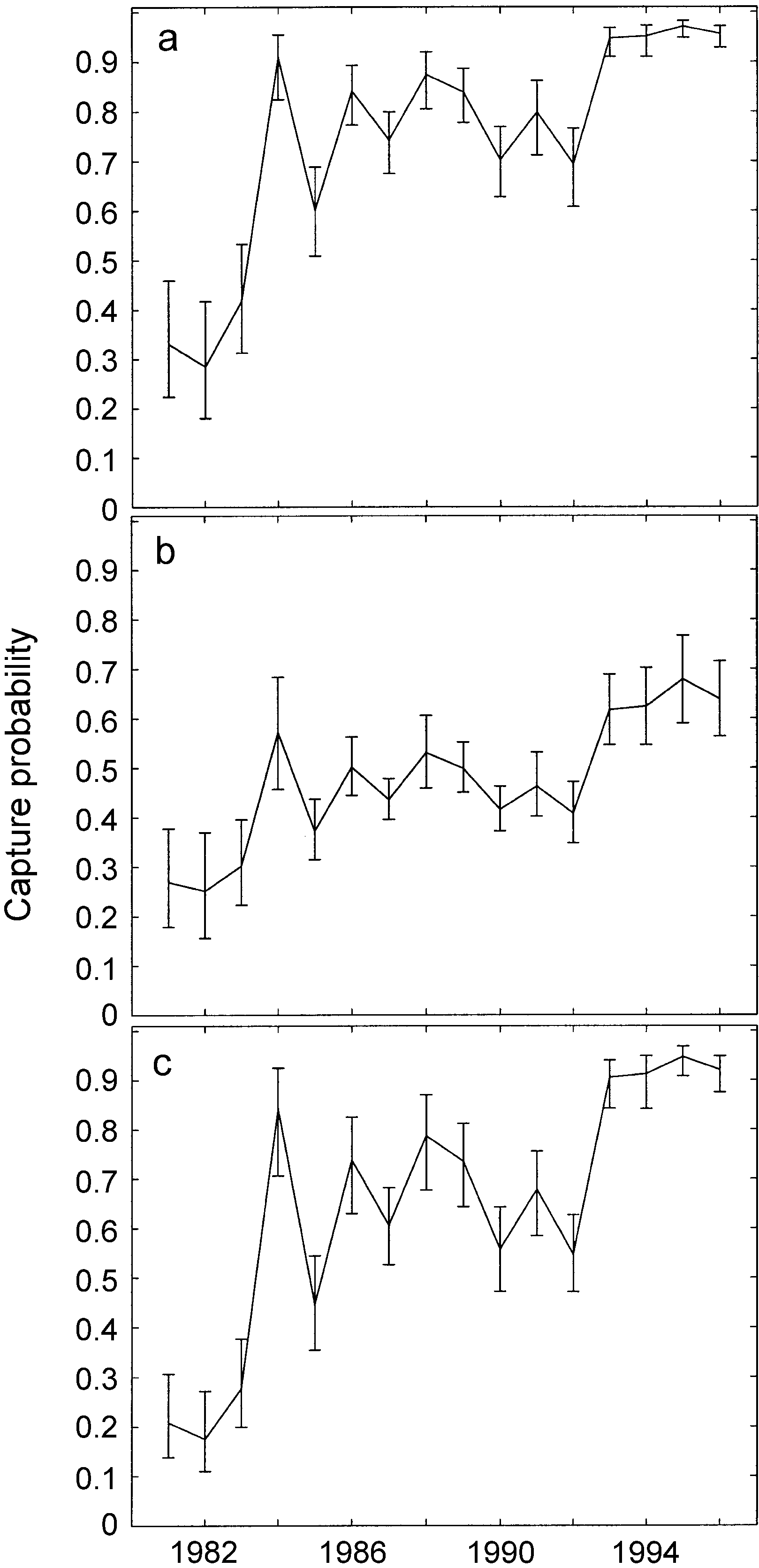 Dependence of the best capture model for the
North Atlantic right whale on effort level and time.
Dependence of the best capture model for the
North Atlantic right whale on effort level and time.